恒等映射，残差神经网络的核心思想

模型退化

随着神经网络的不断发展，越来越深的网络层在现代硬件的加持下成为了可能，并且也切实带来了更好的训练效果。深度学习的研究者们致力于增加和尝试不同的网络、构建更深的网络来尝试获得更好的结果，为了取得质的突破。

然而事与愿违，神经网络似乎并不是越深越好，人们发现当模型层数增加到某种程度，模型的效果将会不升反降。也就是说，深度模型发生了退化（degradation）。

这种退化与以往的过拟合、梯度消失或爆炸问题有着本质的不同。

有推测说，神经网络越来越深的时候，反传回来的梯度之间的相关性会越来越差，最后接近白噪声。因为我们知道图像是具备局部相关性的，那其实可以认为梯度也应该具备类似的相关性，这样更新的梯度才有意义，如果梯度接近白噪声，那梯度更新可能根本就是在做随机扰动。（The Shattered Gradients Problem: If resnets are the answer, then what is the question?）

还有一种理解，层数的增加会扩大解空间，使得结果接近最优解的可能性降低。

总而言之，各类激活函数和网络的构造给了模型足够的灵活性，而越多的网络层反而让模型“忘记了初心”。

恒等映射

按理说，当我们堆叠一个模型时，理所当然的会认为效果会越堆越好。因为，假设一个比较浅的网络已经可以达到不错的效果，那么即使之后堆上去的网络什么也不做，模型的效果也不会变差。

然而事实上，这却是问题所在。“ 什么都不做 ”恰好是当前神经网络最难做到的东西之一。

对应模型这种偏离最优映射的情况，可以用函数族来形式化地说明。

函数族

假设有⼀类特定的神经⽹络架构（函数族）$\cal F$，它包括学习速率和其他超参数设置。

对于任意$f ∈ \cal F$，它总能通过在合适的数据集上进⾏训练⽽确定出合适的参数集，特定的参数集就能将$\cal F$ 具体到$f$。

若$f^∗$ 是我们真正想要找到的函数（在数据集上表现是最好的），那么
当$f^∗∈ \cal F$ 时，我们可以就直接通过训练$\cal F$ 得到它。但通常我们不会那么幸运，我们训练往往只会得到⼀个函数$f^∗_{\cal F}\in{\cal F}$，这是我们在$\cal F$ 中搜索得到的最佳选择，即：

$$f^*_{\cal F}=\arg\min_{f\in\cal F}{\cal L}(\mathbf{X,y}|f)$$

那么，怎样得到更接近最优表现$f^∗$ 的函数呢？唯⼀合理的可能性是，我们需要设计⼀个更强⼤的架构$\cal F'$ 。

理论推导将表明，如果$\cal F'\not\subseteq\cal F$，就⽆法保证新的体系“更接近”最优，甚至更遭。

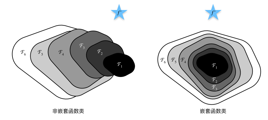
如图所示，对于非嵌套函数（non-nested function）族，越复杂的函数类并不总是向“真”函数靠拢（设复杂度由$\cal F_1$ 向$\cal F_6$ 递增）。相反对于右侧的嵌套函数（nested function）族：$\cal F_1 ⊆ \cdots ⊆ F_6$，可以在复杂度增加的同时，在不偏离原来的解空间的情况下，慢慢接近目标函数。

不断加深网络层，因为激活函数的非线性等问题，就相当于得到了一系列非嵌套函数族的网络框架。而我们的目标就是想办法得到完全包含浅层网络的深层网络，形成嵌套函数族。

残差神经网络

残差设计

针对这上述问题，何恺明等⼈提出了残差⽹络（ResNet）。它在2015年的ImageNet图像识别挑战赛夺魁，并深刻影响了后来的深度神经⽹络的设计。

ResNet的核心思想就是，在浅层网络的基础上，保证新增加的网络层只学习恒等映射。(identity function)

即保证第$L$ 层网络的输出$f(\boldsymbol X)=\boldsymbol X$，其中$\boldsymbol X$ 是第$L-1$ 层的输出。

如果实现了这样的恒等映射，那么无论添加多少层我都能保证深层网络的结果与浅层网络的结果一致！
虽然这看似用处不大，但实际上因为神经网络的灵活性，模型输出自然会在此基础上发散，也就是符合了前面提到的嵌套函数族结构。

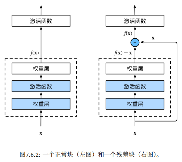
而让一个神经网络层学习恒等映射是很困难的，不过！ 学习残差却容易得多！

我们让第$L$ 层的网络学习$h_L(\boldsymbol x_{L-1})=f(\boldsymbol x_{L-1})-\boldsymbol x_{L-1}$，最后再在此基础上加上$\boldsymbol x_{L-1}$ 本身，最后通过激活函数得到$\boldsymbol x_{L}$，即：

$$\boldsymbol x_{L}=\text{ReLU}\left(h_L(\boldsymbol x_{L-1})+\boldsymbol x_{L-1}\right)$$

忽略激活函数的话，根据递推关系就有：

$$\boldsymbol x_{L}=\boldsymbol x_{1}+\sum_{l=1}^{L-1}h_l(\boldsymbol x_{l})$$

其中，$\boldsymbol x_{1}$ 是浅层网络的输出，即没有残差结构的最后一个网络。

利用链式法则得出：

$$\frac{\partial \cal L}{\partial x_1}=\frac{\partial \cal L}{\partial x_L}\cdot\frac{\partial x_L}{\partial x_1}=\frac{\partial \cal L}{\partial x_L}\cdot\left(1+\sum_{l=1}^{L-1}\frac{\partial h(x_l)}{\partial x_1}\right)$$

可见，有着括号中$1$ 的存在，使得残差网络的梯度不容易消失，并且模型容易学习。

于是乎，这样通过 shortcut connection 进行跨层数据通路的神经网络被设计了出来：

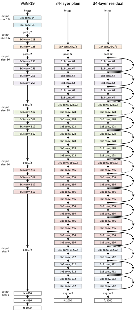
残差块和总体结构

ResNet沿⽤了VGG完整的3 × 3卷积层设计。
残差块⾥⾸先有2个有相同输出通道数的3 × 3卷积层。每个卷积层后接⼀个BN层和ReLU激活函数。
然后通过跨层数据通路，跳过这2个卷积运算，将输⼊直接加在最后的ReLU激活函数前。这样的设计要求2个卷积层的输出与输⼊形状⼀致，从⽽使它们可以相加。
如果想改变通道数，就需要引⼊⼀个额外的1 × 1卷积层来将输⼊变换成需要的形状后再做相加运算。

ResNet整体的网络结构如下图所示，足见它比此前足够深的 VGG-19 还要深。

PyTorch实现

model.py

#model.py

import torch.nn as nn
import torch

#18/34
class BasicBlock(nn.Module):
    expansion = 1 #每一个conv的卷积核个数的倍数

    def __init__(self, in_channel, out_channel, stride=1, downsample=None):#downsample对应虚线残差结构
        super(BasicBlock, self).__init__()
        self.conv1 = nn.Conv2d(in_channels=in_channel, out_channels=out_channel,
                               kernel_size=3, stride=stride, padding=1, bias=False)
        self.bn1 = nn.BatchNorm2d(out_channel)#BN处理
        self.relu = nn.ReLU()
        self.conv2 = nn.Conv2d(in_channels=out_channel, out_channels=out_channel,
                               kernel_size=3, stride=1, padding=1, bias=False)
        self.bn2 = nn.BatchNorm2d(out_channel)
        self.downsample = downsample

    def forward(self, x):
        identity = x #捷径上的输出值
        if self.downsample is not None:
            identity = self.downsample(x)

        out = self.conv1(x)
        out = self.bn1(out)
        out = self.relu(out)

        out = self.conv2(out)
        out = self.bn2(out)

        out += identity
        out = self.relu(out)

        return out

#50,101,152
class Bottleneck(nn.Module):
    expansion = 4#4倍

    def __init__(self, in_channel, out_channel, stride=1, downsample=None):
        super(Bottleneck, self).__init__()
        self.conv1 = nn.Conv2d(in_channels=in_channel, out_channels=out_channel,
                               kernel_size=1, stride=1, bias=False)  # squeeze channels
        self.bn1 = nn.BatchNorm2d(out_channel)
        self.relu = nn.ReLU(inplace=True)
        # -----------------------------------------
        self.conv2 = nn.Conv2d(in_channels=out_channel, out_channels=out_channel,
                               kernel_size=3, stride=stride, bias=False, padding=1)
        self.bn2 = nn.BatchNorm2d(out_channel)
        self.relu = nn.ReLU(inplace=True)
        # -----------------------------------------
        self.conv3 = nn.Conv2d(in_channels=out_channel, out_channels=out_channel*self.expansion,#输出*4
                               kernel_size=1, stride=1, bias=False)  # unsqueeze channels
        self.bn3 = nn.BatchNorm2d(out_channel*self.expansion)
        self.relu = nn.ReLU(inplace=True)
        self.downsample = downsample

    def forward(self, x):
        identity = x
        if self.downsample is not None:
            identity = self.downsample(x)

        out = self.conv1(x)
        out = self.bn1(out)
        out = self.relu(out)

        out = self.conv2(out)
        out = self.bn2(out)
        out = self.relu(out)

        out = self.conv3(out)
        out = self.bn3(out)

        out += identity
        out = self.relu(out)

        return out


class ResNet(nn.Module):

    def __init__(self, block, blocks_num, num_classes=1000, include_top=True):#block残差结构 include_top为了之后搭建更加复杂的网络
        super(ResNet, self).__init__()
        self.include_top = include_top
        self.in_channel = 64

        self.conv1 = nn.Conv2d(3, self.in_channel, kernel_size=7, stride=2,
                               padding=3, bias=False)
        self.bn1 = nn.BatchNorm2d(self.in_channel)
        self.relu = nn.ReLU(inplace=True)
        self.maxpool = nn.MaxPool2d(kernel_size=3, stride=2, padding=1)
        self.layer1 = self._make_layer(block, 64, blocks_num[0])
        self.layer2 = self._make_layer(block, 128, blocks_num[1], stride=2)
        self.layer3 = self._make_layer(block, 256, blocks_num[2], stride=2)
        self.layer4 = self._make_layer(block, 512, blocks_num[3], stride=2)
        if self.include_top:
            self.avgpool = nn.AdaptiveAvgPool2d((1, 1))  # output size = (1, 1)自适应
            self.fc = nn.Linear(512 * block.expansion, num_classes)

        for m in self.modules():
            if isinstance(m, nn.Conv2d):
                nn.init.kaiming_normal_(m.weight, mode='fan_out', nonlinearity='relu')

    def _make_layer(self, block, channel, block_num, stride=1):
        downsample = None
        if stride != 1 or self.in_channel != channel * block.expansion:
            downsample = nn.Sequential(
                nn.Conv2d(self.in_channel, channel * block.expansion, kernel_size=1, stride=stride, bias=False),
                nn.BatchNorm2d(channel * block.expansion))

        layers = []
        layers.append(block(self.in_channel, channel, downsample=downsample, stride=stride))
        self.in_channel = channel * block.expansion

        for _ in range(1, block_num):
            layers.append(block(self.in_channel, channel))

        return nn.Sequential(*layers)

    def forward(self, x):
        x = self.conv1(x)
        x = self.bn1(x)
        x = self.relu(x)
        x = self.maxpool(x)

        x = self.layer1(x)
        x = self.layer2(x)
        x = self.layer3(x)
        x = self.layer4(x)

        if self.include_top:
            x = self.avgpool(x)
            x = torch.flatten(x, 1)
            x = self.fc(x)

        return x


def resnet34(num_classes=1000, include_top=True):
    return ResNet(BasicBlock, [3, 4, 6, 3], num_classes=num_classes, include_top=include_top)


def resnet101(num_classes=1000, include_top=True):
    return ResNet(Bottleneck, [3, 4, 23, 3], num_classes=num_classes, include_top=include_top)

train.py

#train.py

import torch
import torch.nn as nn
from torchvision import transforms, datasets
import json
import matplotlib.pyplot as plt
import os
import torch.optim as optim
from model import resnet34, resnet101
import torchvision.models.resnet


device = torch.device("cuda:0" if torch.cuda.is_available() else "cpu")
print(device)

data_transform = {
    "train": transforms.Compose([transforms.RandomResizedCrop(224),
                                 transforms.RandomHorizontalFlip(),
                                 transforms.ToTensor(),
                                 transforms.Normalize([0.485, 0.456, 0.406], [0.229, 0.224, 0.225])]),#来自官网参数
    "val": transforms.Compose([transforms.Resize(256),#将最小边长缩放到256
                               transforms.CenterCrop(224),
                               transforms.ToTensor(),
                               transforms.Normalize([0.485, 0.456, 0.406], [0.229, 0.224, 0.225])])}


data_root = os.getcwd()
image_path = data_root + "/flower_data/"  # flower data set path

train_dataset = datasets.ImageFolder(root=image_path + "train",
                                     transform=data_transform["train"])
train_num = len(train_dataset)

# {'daisy':0, 'dandelion':1, 'roses':2, 'sunflower':3, 'tulips':4}
flower_list = train_dataset.class_to_idx
cla_dict = dict((val, key) for key, val in flower_list.items())
# write dict into json file
json_str = json.dumps(cla_dict, indent=4)
with open('class_indices.json', 'w') as json_file:
    json_file.write(json_str)

batch_size = 16
train_loader = torch.utils.data.DataLoader(train_dataset,
                                           batch_size=batch_size, shuffle=True,
                                           num_workers=0)

validate_dataset = datasets.ImageFolder(root=image_path + "/val",
                                        transform=data_transform["val"])
val_num = len(validate_dataset)
validate_loader = torch.utils.data.DataLoader(validate_dataset,
                                              batch_size=batch_size, shuffle=False,
                                              num_workers=0)
#net = resnet34()
net = resnet34(num_classes=5)
# load pretrain weights

# model_weight_path = "./resnet34-pre.pth"
# missing_keys, unexpected_keys = net.load_state_dict(torch.load(model_weight_path), strict=False)#载入模型参数

# for param in net.parameters():
#     param.requires_grad = False
# change fc layer structure

# inchannel = net.fc.in_features
# net.fc = nn.Linear(inchannel, 5)


net.to(device)

loss_function = nn.CrossEntropyLoss()
optimizer = optim.Adam(net.parameters(), lr=0.0001)

best_acc = 0.0
save_path = './resNet34.pth'
for epoch in range(3):
    # train
    net.train()
    running_loss = 0.0
    for step, data in enumerate(train_loader, start=0):
        images, labels = data
        optimizer.zero_grad()
        logits = net(images.to(device))
        loss = loss_function(logits, labels.to(device))
        loss.backward()
        optimizer.step()

        # print statistics
        running_loss += loss.item()
        # print train process
        rate = (step+1)/len(train_loader)
        a = "*" * int(rate * 50)
        b = "." * int((1 - rate) * 50)
        print("\rtrain loss: {:^3.0f}%[{}->{}]{:.4f}".format(int(rate*100), a, b, loss), end="")
    print()

    # validate
    net.eval()
    acc = 0.0  # accumulate accurate number / epoch
    with torch.no_grad():
        for val_data in validate_loader:
            val_images, val_labels = val_data
            outputs = net(val_images.to(device))  # eval model only have last output layer
            # loss = loss_function(outputs, test_labels)
            predict_y = torch.max(outputs, dim=1)[1]
            acc += (predict_y == val_labels.to(device)).sum().item()
        val_accurate = acc / val_num
        if val_accurate > best_acc:
            best_acc = val_accurate
            torch.save(net.state_dict(), save_path)
        print('[epoch %d] train_loss: %.3f  test_accuracy: %.3f' %
              (epoch + 1, running_loss / step, val_accurate))

print('Finished Training')

predict.py

#predict.py

import torch
from model import resnet34
from PIL import Image
from torchvision import transforms
import matplotlib.pyplot as plt
import json

data_transform = transforms.Compose(
    [transforms.Resize(256),
     transforms.CenterCrop(224),
     transforms.ToTensor(),
     transforms.Normalize([0.485, 0.456, 0.406], [0.229, 0.224, 0.225])])

# load image
img = Image.open("./roses.jpg")
plt.imshow(img)
# [N, C, H, W]
img = data_transform(img)
# expand batch dimension
img = torch.unsqueeze(img, dim=0)

# read class_indict
try:
    json_file = open('./class_indices.json', 'r')
    class_indict = json.load(json_file)
except Exception as e:
    print(e)
    exit(-1)

# create model
model = resnet34(num_classes=5)
# load model weights
model_weight_path = "./resNet34.pth"
model.load_state_dict(torch.load(model_weight_path))
model.eval()
with torch.no_grad():
    # predict class
    output = torch.squeeze(model(img))
    predict = torch.softmax(output, dim=0)
    predict_cla = torch.argmax(predict).numpy()
print(class_indict[str(predict_cla)], predict[predict_cla].numpy())
plt.show()

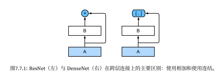
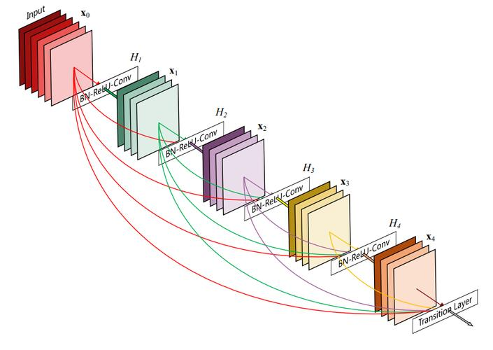
稠密连接网络

吸收了 ResNet 的优点，稠密连接网络（DenseNet） 在保证网络中层与层之间最大程度的信息传输的前提下，直接将所有层连接起来。为了能够保证前馈的特性，每一层将之前所有层的输入进行拼接，之后将输出的特征图传递给之后的所有层。

DenseNet这个名字由变量之间的“稠密连接”⽽得来，最后⼀层与之前的所有层紧密相连。

这样做有几个好处：缓解梯度消失问题、强化feature传递、鼓励feature再利用、极大减少参数总数量（这一点违反直觉，但实际上DenseNet的设计可以避免重复学习feature map；并且网络每一层的通道数非常少）。

此外，整个稠密连接⽹络主要由2部分构成：稠密块（dense block）和过渡层（transition layer）。前者定义如何连接输⼊和输出，⽽后者则通过 1×1 卷积层来控制通道数量，用池化层来减半高和宽，使其不会太复杂。

参考

1. 动手学习深度学习|D2L Discussion - Dive into Deep Learning
2. Resnet到底在解决一个什么问题呢？ - 知乎
3. DenseNet：密集连接卷积网络 - 简书
4. ResNet——CNN经典网络模型详解(pytorch实现)-CSDN博客