Intro 清晨的咖啡杯中,奶精与黑咖啡的交融是一场微观世界的扩散(Diffusion)。无序的布朗运动将奶滴打散,直至达成均匀的混沌——这是热力学第二定律的具象化:熵增不可逆 。 但是如果有一种像电影《信条(TENET)》那样的时间钳形装置,我们或许就能看到奶精和咖啡重新分离回归原位的奇观,熵减了!
破坏一样东西总比创造它容易得多,但是我们是否可以构建一种模型,这个模型能够学习到如何将数据一步步破坏,然后反过来通过反变换将它一步步从被破坏后的样子还原回来呢?这种模型正是一种生成式模型 的新思路, Diffusion Models 就是该思想的贡献者之一,始于2020年所提出的DDPM (Denoising Diffusion Probabilistic Model)。
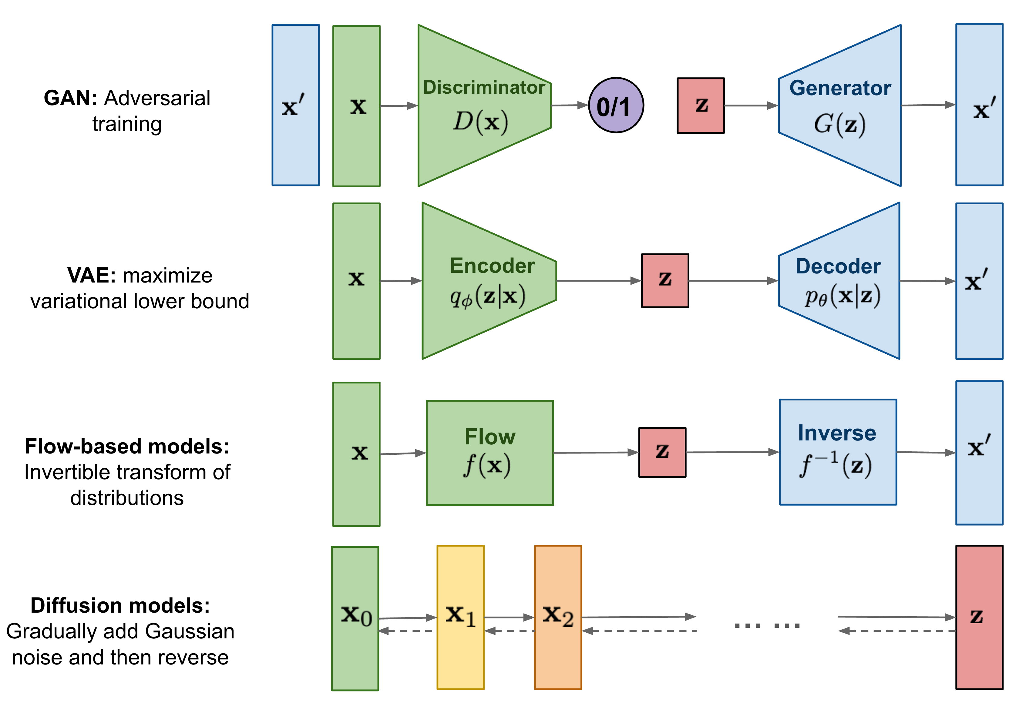
和我们之前介绍的 VAE、GAN 不同,Diffusion models 将原始输入样本x 0 \mathbf x_0 x 0 高斯噪声 (称为前向扩散过程),最终得到z \bf z z 生成 需求。
原理推导 (DDPM) 前向扩散 对于服从真实分布的样本x 0 ∼ q ( x ) \mathbf x_0\sim q(\mathbf x) x 0 ∼ q ( x ) forward diffusion process )被定义为将x 0 \mathbf x_0 x 0 T T T x 1 , … , x T \mathbf{x}_1, \dots, \mathbf{x}_T x 1 , … , x T { β t ∈ ( 0 , 1 ) } t = 1 T \{\beta_t \in (0, 1)\}_{t=1}^T { β t ∈ ( 0 , 1 ) } t = 1 T
q ( x t ∣ x t − 1 ) = N ( x t ; 1 − β t x t − 1 , β t I ) , q ( x 1 : T ∣ x 0 ) = ∏ t = 1 T q ( x t ∣ x t − 1 ) q(\mathbf{x}_t \vert \mathbf{x}_{t-1}) = \mathcal{N}(\mathbf{x}_t; \sqrt{1 - \beta_t} \mathbf{x}_{t-1}, \beta_t\mathbf{I}), \quad q(\mathbf{x}_{1:T} \vert \mathbf{x}_0) = \prod^T_{t=1} q(\mathbf{x}_t \vert \mathbf{x}_{t-1}) q ( x t ∣ x t − 1 ) = N ( x t ; 1 − β t x t − 1 , β t I ) , q ( x 1 : T ∣ x 0 ) = t = 1 ∏ T q ( x t ∣ x t − 1 )
当T → ∞ T\to\infty T → ∞ x T \mathbf x_T x T isotropic Gaussian distribution ,也叫球形高斯分布),即各个方向(每一维度)的方差都相等(Σ = σ I \Sigma=\sigma\bf I Σ = σ I
上面这个公式给出了已知x t − 1 \mathbf x_{t-1} x t − 1 x t \mathbf x_t x t 吓人 ,但是我们可以稍微推导一下:
x t ∼ N ( 1 − β t x t − 1 , β t I ) x t − 1 − β t x t − 1 ∼ N ( 0 , β t I ) ( x t − 1 − β t x t − 1 ) / β t ∼ N ( 0 , I ) \begin{aligned} \mathbf x_t&\sim \mathcal{N}(\sqrt{1 - \beta_t} \mathbf{x}_{t-1}, \beta_t\mathbf{I})\\ \mathbf x_t-\sqrt{1 - \beta_t} \mathbf{x}_{t-1} &\sim \mathcal{N}(0, \beta_t\mathbf{I})\\ \big(\mathbf x_t-\sqrt{1 - \beta_t} \mathbf{x}_{t-1}\big)/\sqrt{\beta_t} &\sim \mathcal{N}(0, \mathbf{I}) \end{aligned} x t x t − 1 − β t x t − 1 ( x t − 1 − β t x t − 1 ) / β t ∼ N ( 1 − β t x t − 1 , β t I ) ∼ N ( 0 , β t I ) ∼ N ( 0 , I )
令ϵ t − 1 ∼ N ( 0 , I ) \mathbf\epsilon_{t-1}\sim\mathcal N(0,\mathbf I) ϵ t − 1 ∼ N ( 0 , I ) x t \mathbf x_t x t x t − 1 \mathbf x_{t-1} x t − 1 ϵ t − 1 \mathbf\epsilon_{t-1} ϵ t − 1
x t = 1 − β t x t − 1 + β t ϵ t − 1 \mathbf x_t=\sqrt{1 - \beta_t} \mathbf{x}_{t-1}+\sqrt{\beta_t}\boldsymbol{\epsilon}_{t-1} x t = 1 − β t x t − 1 + β t ϵ t − 1
这个显式的递推公式 还可以指导我们直接一步到位推导出x t \mathbf x_t x t x t − 2 \mathbf x_{t-2} x t − 2 α t = 1 − β t \alpha_t=1-\beta_t α t = 1 − β t
x t = 1 − β t x t − 1 + β t ϵ 1 = α t x t − 1 + 1 − α t ϵ 1 = α t ( α t − 1 x t − 2 + 1 − α t − 1 ϵ 2 ) + 1 − α t ϵ 1 = α t α 1 x 2 + α t 1 − α t − 1 ϵ 2 + 1 − α t ϵ 1 = α t α 1 x 2 + 1 − α t α 1 ϵ ˉ 2 where ϵ ˉ 2 ∼ N ( 0 , I ) ∗ Tips N ( 0 , σ 1 2 I ) + N ( 0 , σ 2 2 I ) = N ( 0 , ( σ 1 2 + σ 2 2 ) I ) \begin{aligned} \mathbf x_t&=\sqrt{1 - \beta_t} \mathbf{x}_{t-1}+\sqrt{\beta_t}\boldsymbol{\epsilon}_{1}\\ &=\sqrt{\alpha_t}\mathbf{x}_{t-1}+\sqrt{1-\alpha_t}\boldsymbol{\epsilon}_{1}\\ &=\sqrt{\alpha_t}\big(\sqrt{\alpha_{t-1}}\mathbf x_{t-2}+\sqrt{1-\alpha_{t-1}}\boldsymbol{\epsilon}_{2}\big)+\sqrt{1-\alpha_t}\boldsymbol{\epsilon}_{1}\\ &=\sqrt{\alpha_t\alpha_{1}}\mathbf x_{2}+\sqrt{\alpha_t}\sqrt{1-\alpha_{t-1}}\boldsymbol{\epsilon}_{2}+\sqrt{1-\alpha_t}\boldsymbol{\epsilon}_{1}\\ &=\sqrt{\alpha_t\alpha_{1}}\mathbf x_{2}+\sqrt{1-\alpha_t\alpha_{1}}\bar{\boldsymbol{\epsilon}}_{2} \quad\text{where }\bar{\boldsymbol{\epsilon}}_{2}\sim\mathcal{N}(0,\mathbf I) \\\\ &^{*\text{Tips}}\;\mathcal{N}(0,\sigma_1^2\mathbf I)+\mathcal{N}(0,\sigma_2^2\mathbf I)=\mathcal{N}\big(0,(\sigma_1^2+\sigma_2^2)\mathbf I\big) \end{aligned} x t = 1 − β t x t − 1 + β t ϵ 1 = α t x t − 1 + 1 − α t ϵ 1 = α t ( α t − 1 x t − 2 + 1 − α t − 1 ϵ 2 ) + 1 − α t ϵ 1 = α t α 1 x 2 + α t 1 − α t − 1 ϵ 2 + 1 − α t ϵ 1 = α t α 1 x 2 + 1 − α t α 1 ϵ ˉ 2 where ϵ ˉ 2 ∼ N ( 0 , I ) ∗ Tips N ( 0 , σ 1 2 I ) + N ( 0 , σ 2 2 I ) = N ( 0 , ( σ 1 2 + σ 2 2 ) I )
更进一步地,令α ˉ t = ∏ i = 1 t α i \bar{\alpha}_t = \prod_{i=1}^t \alpha_i α ˉ t = ∏ i = 1 t α i x t \mathbf x_t x t x 0 \mathbf x_{0} x 0
x t = α ˉ t x 0 + 1 − α ˉ t ϵ t ( ⋆ ) i . e . q ( x t ∣ x 0 ) = N ( x t ; α ˉ t x 0 , ( 1 − α ˉ t ) I ) \begin{aligned} \mathbf{x}_t &= \sqrt{\bar{\alpha}_t}\mathbf{x}_0 + \sqrt{1 - \bar{\alpha}_t}\boldsymbol{\epsilon}_t \quad(\star)\\ i.e.\;q(\mathbf{x}_t \vert \mathbf{x}_0) &= \mathcal{N}(\mathbf{x}_t; \sqrt{\bar{\alpha}_t} \mathbf{x}_0, (1 - \bar{\alpha}_t)\mathbf{I}) \end{aligned} x t i . e . q ( x t ∣ x 0 ) = α ˉ t x 0 + 1 − α ˉ t ϵ t ( ⋆ ) = N ( x t ; α ˉ t x 0 , ( 1 − α ˉ t ) I )
反过来,有:
x 0 = 1 α ˉ t x t − 1 α ˉ t − 1 ϵ t ( ⋆ ) \mathbf{x}_0=\sqrt{\frac1{\bar{\alpha}_t}}\;\mathbf{x}_t-\sqrt{\frac1{\bar{\alpha}_t}-1}\;\boldsymbol{\epsilon}_t\quad(\star) x 0 = α ˉ t 1 x t − α ˉ t 1 − 1 ϵ t ( ⋆ )
通常,当样本被加噪变得更嘈杂时,其可以负担得起更大的更新步骤,所以有β 1 < β 2 < ⋯ < β T \beta_1 < \beta_2 < \dots < \beta_T β 1 < β 2 < ⋯ < β T α ˉ 1 > ⋯ > α ˉ T \bar{\alpha}_1 > \dots > \bar{\alpha}_T α ˉ 1 > ⋯ > α ˉ T
反向扩散 一个很直观的想法就是,既然x t \mathbf x_{t} x t α t x t − 1 + 1 − α t ϵ 1 \sqrt{\alpha_t}\mathbf{x}_{t-1}+\sqrt{1-\alpha_t}\boldsymbol{\epsilon}_{1} α t x t − 1 + 1 − α t ϵ 1 x t − 1 \mathbf x_{t-1} x t − 1
x t − 1 = x t − 1 − α t ϵ 1 α t \mathbf x_{t-1}=\frac{\mathbf x_{t}-\sqrt{1-\alpha_t}\boldsymbol{\epsilon}_{1}}{\sqrt{\alpha_{t}}} x t − 1 = α t x t − 1 − α t ϵ 1
所以如果我们需要学习一个从x t \mathbf x_{t} x t x t − 1 \mathbf x_{t-1} x t − 1 μ θ ( x t , t ) \boldsymbol\mu_\theta(\mathbf x_{t},t) μ θ ( x t , t ) ϵ t − 1 \boldsymbol{\epsilon}_{t-1} ϵ t − 1
∥ x t − 1 − μ θ ( x t , t ) ∥ 2 \Vert\mathbf x_{t-1}-\boldsymbol\mu_\theta(\mathbf x_{t},t)\Vert^2 ∥ x t − 1 − μ θ ( x t , t ) ∥ 2
其实它就等价于优化:
∥ ϵ 1 − ϵ θ ( x t , t ) ∥ 2 \Vert\boldsymbol\epsilon_{1}-\boldsymbol\epsilon_\theta(\mathbf x_{t},t)\Vert^2 ∥ ϵ 1 − ϵ θ ( x t , t ) ∥ 2
更进一步地,在训练模型时x 0 \mathbf x_0 x 0 x 0 \mathbf x_0 x 0 x t \mathbf x_t x t t t t 积分技巧 将多次采用的ϵ t \boldsymbol{\epsilon}_t ϵ t ϵ \boldsymbol{\epsilon} ϵ 苏剑林老师 在其博客
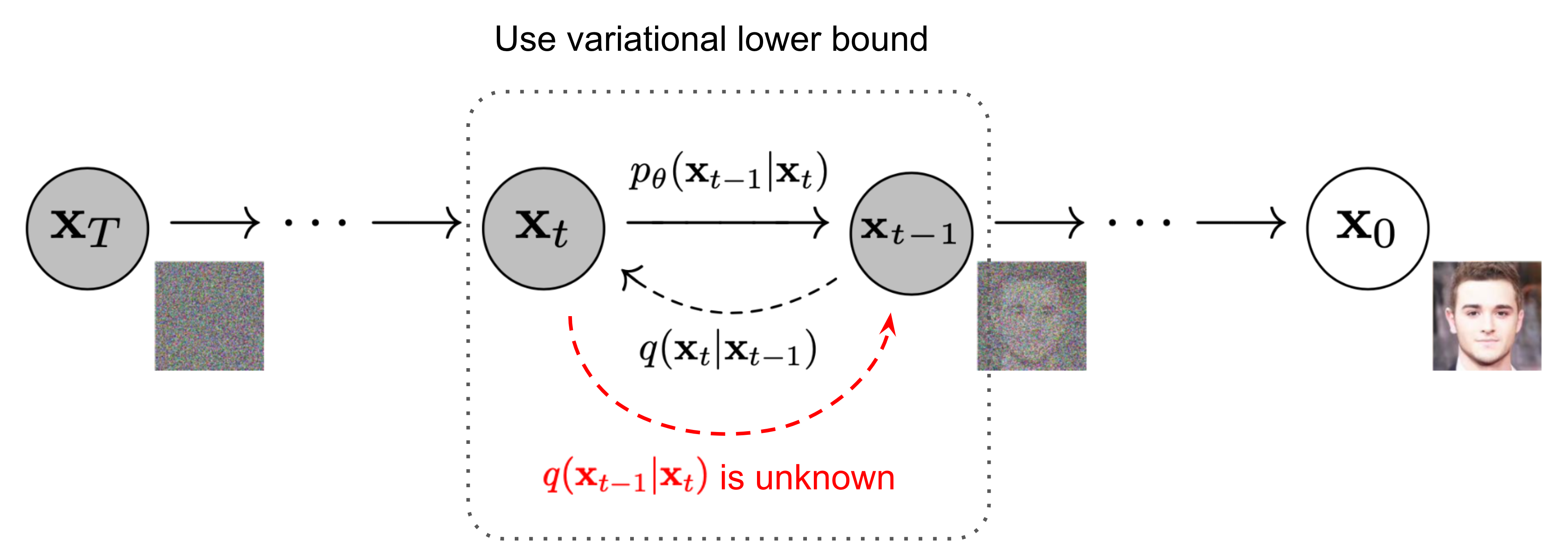
如果用概率学的写法(毕竟原文就自称扩散概率 模型),我们的目标是要拟合出从x t \mathbf x_{t} x t x t − 1 \mathbf x_{t-1} x t − 1
p θ ( x t − 1 ∣ x t ) = N ( x t − 1 ; μ θ ( x t , t ) , Σ θ ( x t , t ) ) p θ ( x 0 : T ) = p ( x T ) ∏ t = 1 T p θ ( x t − 1 ∣ x t ) \begin{aligned} p_\theta(\mathbf{x}_{t-1} \vert \mathbf{x}_t) &= \mathcal{N}(\mathbf{x}_{t-1}; \boldsymbol{\mu}_\theta(\mathbf{x}_t, t), \boldsymbol{\Sigma}_\theta(\mathbf{x}_t, t))\\ p_\theta(\mathbf{x}_{0:T}) &= p(\mathbf{x}_T) \prod^T_{t=1} p_\theta(\mathbf{x}_{t-1} \vert \mathbf{x}_t) \end{aligned} p θ ( x t − 1 ∣ x t ) p θ ( x 0 : T ) = N ( x t − 1 ; μ θ ( x t , t ) , Σ θ ( x t , t )) = p ( x T ) t = 1 ∏ T p θ ( x t − 1 ∣ x t )
要达成这个目的,前提是先知道在现实分布q ( ⋅ ) q(\cdot) q ( ⋅ ) q ( x t − 1 ∣ x t ) q(\mathbf{x}_{t-1} \vert \mathbf{x}_t) q ( x t − 1 ∣ x t )
有文献指出如果 q ( x t ∣ x t − 1 ) q(\mathbf{x}_{t} \vert \mathbf{x}_{t-1}) q ( x t ∣ x t − 1 ) β t \beta_t β t q ( x t − 1 ∣ x t ) q(\mathbf{x}_{t-1} \vert \mathbf{x}_t) q ( x t − 1 ∣ x t ) q ( x t − 1 ∣ x t ) q(\mathbf{x}_{t-1} \vert \mathbf{x}_t) q ( x t − 1 ∣ x t ) x 0 \mathbf x_0 x 0 x 0 \mathbf x_0 x 0 q ( x t − 1 ∣ x t , x 0 ) q(\mathbf{x}_{t-1} \vert \mathbf{x}_t, \mathbf{x}_0) q ( x t − 1 ∣ x t , x 0 )
q ( x t − 1 ∣ x t , x 0 ) = N ( x t − 1 ; μ ~ ( x t , x 0 ) , β ~ t I ) q(\mathbf{x}_{t-1} \vert \mathbf{x}_t, \mathbf{x}_0) = \mathcal{N}(\mathbf{x}_{t-1}; {\color{blue}{\tilde{\boldsymbol{\mu}}}(\mathbf{x}_t, \mathbf{x}_0)}, {\color{red}{\tilde{\beta}_t} \mathbf{I}}) q ( x t − 1 ∣ x t , x 0 ) = N ( x t − 1 ; μ ~ ( x t , x 0 ) , β ~ t I )
可以利用贝叶斯公式进行推导:
q ( x t − 1 ∣ x t , x 0 ) = q ( x t ∣ x t − 1 , x 0 ) q ( x t − 1 ∣ x 0 ) q ( x t ∣ x 0 ) ∝ exp ( − 1 2 ( ( x t − α t x t − 1 ) 2 β t + ( x t − 1 − α ˉ t − 1 x 0 ) 2 1 − α ˉ t − 1 − ( x t − α ˉ t x 0 ) 2 1 − α ˉ t ) ) = exp ( − 1 2 ( x t 2 − 2 α t x t x t − 1 + α t x t − 1 2 β t + x t − 1 2 − 2 α ˉ t − 1 x 0 x t − 1 + α ˉ t − 1 x 0 2 1 − α ˉ t − 1 − ( x t − α ˉ t x 0 ) 2 1 − α ˉ t ) ) = exp ( − 1 2 ( ( α t β t + 1 1 − α ˉ t − 1 ) x t − 1 2 − ( 2 α t β t x t + 2 α ˉ t − 1 1 − α ˉ t − 1 x 0 ) x t − 1 + C ( x t , x 0 ) ) ) \begin{aligned} q(\mathbf{x}_{t-1} \vert \mathbf{x}_t, \mathbf{x}_0) &= q(\mathbf{x}_t \vert \mathbf{x}_{t-1}, \mathbf{x}_0) \frac{ q(\mathbf{x}_{t-1} \vert \mathbf{x}_0) }{ q(\mathbf{x}_t \vert \mathbf{x}_0) } \\ &\propto \exp \Big(-\frac{1}{2} \big(\frac{(\mathbf{x}_t - \sqrt{\alpha_t} \mathbf{x}_{t-1})^2}{\beta_t} + \frac{(\mathbf{x}_{t-1} - \sqrt{\bar{\alpha}_{t-1}} \mathbf{x}_0)^2}{1-\bar{\alpha}_{t-1}} - \frac{(\mathbf{x}_t - \sqrt{\bar{\alpha}_t} \mathbf{x}_0)^2}{1-\bar{\alpha}_t} \big) \Big) \\ &= \exp \Big(-\frac{1}{2} \big(\frac{\mathbf{x}_t^2 - 2\sqrt{\alpha_t} \mathbf{x}_t {\color{blue}{\mathbf{x}_{t-1}}} + \alpha_t {\color{red}{\mathbf{x}_{t-1}^2}} }{\beta_t} + \frac{ {\color{red}{\mathbf{x}_{t-1}^2}}{- 2 \sqrt{\bar{\alpha}_{t-1}} \mathbf{x}_0} {\color{blue}{\mathbf{x}_{t-1}}}{+ \bar{\alpha}_{t-1} \mathbf{x}_0^2} }{1-\bar{\alpha}_{t-1}} - \frac{(\mathbf{x}_t - \sqrt{\bar{\alpha}_t} \mathbf{x}_0)^2}{1-\bar{\alpha}_t} \big) \Big) \\ &= \exp\Big( -\frac{1}{2} \big( {\color{red}{(\frac{\alpha_t}{\beta_t} + \frac{1}{1 - \bar{\alpha}_{t-1}})} \mathbf{x}_{t-1}^2} - {\color{blue}{(\frac{2\sqrt{\alpha_t}}{\beta_t} \mathbf{x}_t + \frac{2\sqrt{\bar{\alpha}_{t-1}}}{1 - \bar{\alpha}_{t-1}} \mathbf{x}_0)} \mathbf{x}_{t-1}}{ + C(\mathbf{x}_t, \mathbf{x}_0) \big) \Big)} \end{aligned} q ( x t − 1 ∣ x t , x 0 ) = q ( x t ∣ x t − 1 , x 0 ) q ( x t ∣ x 0 ) q ( x t − 1 ∣ x 0 ) ∝ exp ( − 2 1 ( β t ( x t − α t x t − 1 ) 2 + 1 − α ˉ t − 1 ( x t − 1 − α ˉ t − 1 x 0 ) 2 − 1 − α ˉ t ( x t − α ˉ t x 0 ) 2 ) ) = exp ( − 2 1 ( β t x t 2 − 2 α t x t x t − 1 + α t x t − 1 2 + 1 − α ˉ t − 1 x t − 1 2 − 2 α ˉ t − 1 x 0 x t − 1 + α ˉ t − 1 x 0 2 − 1 − α ˉ t ( x t − α ˉ t x 0 ) 2 ) ) = exp ( − 2 1 ( ( β t α t + 1 − α ˉ t − 1 1 ) x t − 1 2 − ( β t 2 α t x t + 1 − α ˉ t − 1 2 α ˉ t − 1 x 0 ) x t − 1 + C ( x t , x 0 ) ) )
其中C ( x t , x 0 ) C(\mathbf{x}_t, \mathbf{x}_0) C ( x t , x 0 ) x t − 1 \mathbf x_{t-1} x t − 1 β ~ t I {\color{red}{\tilde{\beta}_t} \mathbf{I}} β ~ t I μ ~ ( x t , x 0 ) {\color{blue}{\tilde{\boldsymbol{\mu}}}(\mathbf{x}_t, \mathbf{x}_0)} μ ~ ( x t , x 0 )
β ~ t = 1 / ( α t β t + 1 1 − α ˉ t − 1 ) = 1 / ( α t − α ˉ t + β t β t ( 1 − α ˉ t − 1 ) ) = 1 − α ˉ t − 1 1 − α ˉ t ⋅ β t μ ~ t ( x t , x 0 ) = ( α t β t x t + α ˉ t − 1 1 − α ˉ t − 1 x 0 ) / ( α t β t + 1 1 − α ˉ t − 1 ) = ( α t β t x t + α ˉ t − 1 1 − α ˉ t − 1 x 0 ) 1 − α ˉ t − 1 1 − α ˉ t ⋅ β t = α t ( 1 − α ˉ t − 1 ) 1 − α ˉ t x t + α ˉ t − 1 β t 1 − α ˉ t x 0 \begin{aligned} \tilde{\beta}_t &= 1/(\frac{\alpha_t}{\beta_t} + \frac{1}{1 - \bar{\alpha}_{t-1}}) = 1/(\frac{\alpha_t - \bar{\alpha}_t + \beta_t}{\beta_t(1 - \bar{\alpha}_{t-1})}) = {\color{green}{\frac{1 - \bar{\alpha}_{t-1}}{1 - \bar{\alpha}_t} \cdot \beta_t}} \\ \tilde{\boldsymbol{\mu}}_t (\mathbf{x}_t, \mathbf{x}_0) &= (\frac{\sqrt{\alpha_t}}{\beta_t} \mathbf{x}_t + \frac{\sqrt{\bar{\alpha}_{t-1} }}{1 - \bar{\alpha}_{t-1}} \mathbf{x}_0)/(\frac{\alpha_t}{\beta_t} + \frac{1}{1 - \bar{\alpha}_{t-1}}) \\ &= (\frac{\sqrt{\alpha_t}}{\beta_t} \mathbf{x}_t + \frac{\sqrt{\bar{\alpha}_{t-1} }}{1 - \bar{\alpha}_{t-1}} \mathbf{x}_0) {\color{green}{\frac{1 - \bar{\alpha}_{t-1}}{1 - \bar{\alpha}_t} \cdot \beta_t}} \\ &= \frac{\sqrt{\alpha_t}(1 - \bar{\alpha}_{t-1})}{1 - \bar{\alpha}_t} \mathbf{x}_t + \frac{\sqrt{\bar{\alpha}_{t-1}}\beta_t}{1 - \bar{\alpha}_t} \mathbf{x}_0\\ \end{aligned} β ~ t μ ~ t ( x t , x 0 ) = 1/ ( β t α t + 1 − α ˉ t − 1 1 ) = 1/ ( β t ( 1 − α ˉ t − 1 ) α t − α ˉ t + β t ) = 1 − α ˉ t 1 − α ˉ t − 1 ⋅ β t = ( β t α t x t + 1 − α ˉ t − 1 α ˉ t − 1 x 0 ) / ( β t α t + 1 − α ˉ t − 1 1 ) = ( β t α t x t + 1 − α ˉ t − 1 α ˉ t − 1 x 0 ) 1 − α ˉ t 1 − α ˉ t − 1 ⋅ β t = 1 − α ˉ t α t ( 1 − α ˉ t − 1 ) x t + 1 − α ˉ t α ˉ t − 1 β t x 0
此时再将 (★) 式代入,就可以把期望函数改写成
μ ~ t = α t ( 1 − α ˉ t − 1 ) 1 − α ˉ t x t + α ˉ t − 1 β t 1 − α ˉ t 1 α ˉ t ( x t − 1 − α ˉ t ϵ t ) = 1 α t ( x t − 1 − α t 1 − α ˉ t ϵ t ) \begin{aligned} \tilde{\boldsymbol{\mu}}_t &= \frac{\sqrt{\alpha_t}(1 - \bar{\alpha}_{t-1})}{1 - \bar{\alpha}_t} \mathbf{x}_t + \frac{\sqrt{\bar{\alpha}_{t-1}}\beta_t}{1 - \bar{\alpha}_t} \frac{1}{\sqrt{\bar{\alpha}_t}}(\mathbf{x}_t - \sqrt{1 - \bar{\alpha}_t}\boldsymbol{\epsilon}_t) \\ &={\frac{1}{\sqrt{\alpha_t}} \Big( \mathbf{x}_t - \frac{1 - \alpha_t}{\sqrt{1 - \bar{\alpha}_t}} \boldsymbol{\epsilon}_t \Big)} \end{aligned} μ ~ t = 1 − α ˉ t α t ( 1 − α ˉ t − 1 ) x t + 1 − α ˉ t α ˉ t − 1 β t α ˉ t 1 ( x t − 1 − α ˉ t ϵ t ) = α t 1 ( x t − 1 − α ˉ t 1 − α t ϵ t )
这样一来,我们就推导出了真实分布下的q ( x t − 1 ∣ x t , x 0 ) q(\mathbf{x}_{t-1} \vert \mathbf{x}_t, \mathbf{x}_0) q ( x t − 1 ∣ x t , x 0 ) ϵ t \boldsymbol{\epsilon}_t ϵ t
∥ ϵ t − ϵ θ ( x t , t ) ∥ 2 \Vert\boldsymbol\epsilon_{t}-\boldsymbol\epsilon_\theta(\mathbf x_{t},t)\Vert^2 ∥ ϵ t − ϵ θ ( x t , t ) ∥ 2
但是还有一个关键问题,这里是拟合带x 0 \mathbf x_0 x 0 q ( x t − 1 ∣ x t , x 0 ) q(\mathbf{x}_{t-1} \vert \mathbf{x}_t, \mathbf{x}_0) q ( x t − 1 ∣ x t , x 0 ) x 0 \mathbf x_0 x 0 q ( x t − 1 ∣ x t ) q(\mathbf{x}_{t-1} \vert \mathbf{x}_t) q ( x t − 1 ∣ x t )
回归正题,对于一个生成任务来说,我们最终的目的都是为了最大化(边缘)似然 p θ ( x 0 ) p_{\theta}(\mathbf x_0) p θ ( x 0 )
p θ ( x 0 ) = ∫ p θ ( x 0 : T ) d x 1 : T p_{\theta}(\mathbf x_0)=\int p_{\theta}(\mathbf x_{0:T})\mathrm d\mathbf x_{1:T} p θ ( x 0 ) = ∫ p θ ( x 0 : T ) d x 1 : T
这个积分是很难直接去计算的,不过我们可以利用变分下界 (variational lower bound,VLB. 也称 Evidence Lower Bound,ELBO,证据下界),找到p θ ( x 0 ) p_{\theta}(\mathbf x_0) p θ ( x 0 ) 介绍VAE的文章 里也有相关阐释)。
− log p θ ( x 0 ) ≤ − log p θ ( x 0 ) + D KL ( q ( x 1 : T ∣ x 0 ) ∥ p θ ( x 1 : T ∣ x 0 ) ) ; KL is non-negative = − log p θ ( x 0 ) + E x 1 : T ∼ q ( x 1 : T ∣ x 0 ) [ log q ( x 1 : T ∣ x 0 ) p θ ( x 0 : T ) / p θ ( x 0 ) ] = − log p θ ( x 0 ) + E q [ log q ( x 1 : T ∣ x 0 ) p θ ( x 0 : T ) + log p θ ( x 0 ) ] = E q [ log q ( x 1 : T ∣ x 0 ) p θ ( x 0 : T ) ] Let L VLB = E q ( x 0 : T ) [ log q ( x 1 : T ∣ x 0 ) p θ ( x 0 : T ) ] ≥ − E q ( x 0 ) log p θ ( x 0 ) \begin{aligned} - \log p_\theta(\mathbf{x}_0) &\leq - \log p_\theta(\mathbf{x}_0) + D_\text{KL}(q(\mathbf{x}_{1:T}\vert\mathbf{x}_0) \| p_\theta(\mathbf{x}_{1:T}\vert\mathbf{x}_0) ) & \small{\text{; KL is non-negative}}\\ &= - \log p_\theta(\mathbf{x}_0) + \mathbb{E}_{\mathbf{x}_{1:T}\sim q(\mathbf{x}_{1:T} \vert \mathbf{x}_0)} \Big[ \log\frac{q(\mathbf{x}_{1:T}\vert\mathbf{x}_0)}{p_\theta(\mathbf{x}_{0:T}) / p_\theta(\mathbf{x}_0)} \Big] \\ &= - \log p_\theta(\mathbf{x}_0) + \mathbb{E}_q \Big[ \log\frac{q(\mathbf{x}_{1:T}\vert\mathbf{x}_0)}{p_\theta(\mathbf{x}_{0:T})} + \log p_\theta(\mathbf{x}_0) \Big] \\ &= \mathbb{E}_q \Big[ \log \frac{q(\mathbf{x}_{1:T}\vert\mathbf{x}_0)}{p_\theta(\mathbf{x}_{0:T})} \Big] \\ \text{Let }L_\text{VLB} &= \mathbb{E}_{q(\mathbf{x}_{0:T})} \Big[ \log \frac{q(\mathbf{x}_{1:T}\vert\mathbf{x}_0)}{p_\theta(\mathbf{x}_{0:T})} \Big] \geq - \mathbb{E}_{q(\mathbf{x}_0)} \log p_\theta(\mathbf{x}_0) \end{aligned} − log p θ ( x 0 ) Let L VLB ≤ − log p θ ( x 0 ) + D KL ( q ( x 1 : T ∣ x 0 ) ∥ p θ ( x 1 : T ∣ x 0 )) = − log p θ ( x 0 ) + E x 1 : T ∼ q ( x 1 : T ∣ x 0 ) [ log p θ ( x 0 : T ) / p θ ( x 0 ) q ( x 1 : T ∣ x 0 ) ] = − log p θ ( x 0 ) + E q [ log p θ ( x 0 : T ) q ( x 1 : T ∣ x 0 ) + log p θ ( x 0 ) ] = E q [ log p θ ( x 0 : T ) q ( x 1 : T ∣ x 0 ) ] = E q ( x 0 : T ) [ log p θ ( x 0 : T ) q ( x 1 : T ∣ x 0 ) ] ≥ − E q ( x 0 ) log p θ ( x 0 ) ; KL is non-negative
也就是说,我们只需要最小化L VLB L_\text{VLB} L VLB p θ ( x 0 ) p_{\theta}(\mathbf x_0) p θ ( x 0 ) Lil’Log )
更进一步地,这里 VLB 的公式还可以继续展开,把我们前面推导出来的q ( x t − 1 ∣ x t , x 0 ) q(\mathbf{x}_{t-1} \vert \mathbf{x}_t, \mathbf{x}_0) q ( x t − 1 ∣ x t , x 0 )
L VLB = E q ( x 0 : T ) [ log q ( x 1 : T ∣ x 0 ) p θ ( x 0 : T ) ] = E q [ log ∏ t = 1 T q ( x t ∣ x t − 1 ) p θ ( x T ) ∏ t = 1 T p θ ( x t − 1 ∣ x t ) ] = E q [ − log p θ ( x T ) + ∑ t = 1 T log q ( x t ∣ x t − 1 ) p θ ( x t − 1 ∣ x t ) ] = E q [ − log p θ ( x T ) + ∑ t = 2 T log q ( x t ∣ x t − 1 ) p θ ( x t − 1 ∣ x t ) + log q ( x 1 ∣ x 0 ) p θ ( x 0 ∣ x 1 ) ] = E q [ − log p θ ( x T ) + ∑ t = 2 T log ( q ( x t − 1 ∣ x t , x 0 ) p θ ( x t − 1 ∣ x t ) ⋅ q ( x t ∣ x 0 ) q ( x t − 1 ∣ x 0 ) ) + log q ( x 1 ∣ x 0 ) p θ ( x 0 ∣ x 1 ) ] = E q [ − log p θ ( x T ) + ∑ t = 2 T log q ( x t − 1 ∣ x t , x 0 ) p θ ( x t − 1 ∣ x t ) + ∑ t = 2 T log q ( x t ∣ x 0 ) q ( x t − 1 ∣ x 0 ) + log q ( x 1 ∣ x 0 ) p θ ( x 0 ∣ x 1 ) ] = E q [ − log p θ ( x T ) + ∑ t = 2 T log q ( x t − 1 ∣ x t , x 0 ) p θ ( x t − 1 ∣ x t ) + log q ( x T ∣ x 0 ) q ( x 1 ∣ x 0 ) + log q ( x 1 ∣ x 0 ) p θ ( x 0 ∣ x 1 ) ] = E q [ log q ( x T ∣ x 0 ) p θ ( x T ) + ∑ t = 2 T log q ( x t − 1 ∣ x t , x 0 ) p θ ( x t − 1 ∣ x t ) − log p θ ( x 0 ∣ x 1 ) ] = E q [ D KL ( q ( x T ∣ x 0 ) ∥ p θ ( x T ) ) ⏟ L T + ∑ t = 2 T D KL ( q ( x t − 1 ∣ x t , x 0 ) ∥ p θ ( x t − 1 ∣ x t ) ) ⏟ L t − 1 − log p θ ( x 0 ∣ x 1 ) ⏟ L 0 ] \begin{aligned} L_\text{VLB} &= \mathbb{E}_{q(\mathbf{x}_{0:T})} \Big[ \log\frac{q(\mathbf{x}_{1:T}\vert\mathbf{x}_0)}{p_\theta(\mathbf{x}_{0:T})} \Big] \\ &= \mathbb{E}_q \Big[ \log\frac{\prod_{t=1}^T q(\mathbf{x}_t\vert\mathbf{x}_{t-1})}{ p_\theta(\mathbf{x}_T) \prod_{t=1}^T p_\theta(\mathbf{x}_{t-1} \vert\mathbf{x}_t) } \Big] \\ &= \mathbb{E}_q \Big[ -\log p_\theta(\mathbf{x}_T) + \sum_{t=1}^T \log \frac{q(\mathbf{x}_t\vert\mathbf{x}_{t-1})}{p_\theta(\mathbf{x}_{t-1} \vert\mathbf{x}_t)} \Big] \\ &= \mathbb{E}_q \Big[ -\log p_\theta(\mathbf{x}_T) + \sum_{t=2}^T \log \frac{q(\mathbf{x}_t\vert\mathbf{x}_{t-1})}{p_\theta(\mathbf{x}_{t-1} \vert\mathbf{x}_t)} + \log\frac{q(\mathbf{x}_1 \vert \mathbf{x}_0)}{p_\theta(\mathbf{x}_0 \vert \mathbf{x}_1)} \Big] \\ &= \mathbb{E}_q \Big[ -\log p_\theta(\mathbf{x}_T) + \sum_{t=2}^T \log \Big( \frac{q(\mathbf{x}_{t-1} \vert \mathbf{x}_t, \mathbf{x}_0)}{p_\theta(\mathbf{x}_{t-1} \vert\mathbf{x}_t)}\cdot \frac{q(\mathbf{x}_t \vert \mathbf{x}_0)}{q(\mathbf{x}_{t-1}\vert\mathbf{x}_0)} \Big) + \log \frac{q(\mathbf{x}_1 \vert \mathbf{x}_0)}{p_\theta(\mathbf{x}_0 \vert \mathbf{x}_1)} \Big] \\ &= \mathbb{E}_q \Big[ -\log p_\theta(\mathbf{x}_T) + \sum_{t=2}^T \log \frac{q(\mathbf{x}_{t-1} \vert \mathbf{x}_t, \mathbf{x}_0)}{p_\theta(\mathbf{x}_{t-1} \vert\mathbf{x}_t)} + \sum_{t=2}^T \log \frac{q(\mathbf{x}_t \vert \mathbf{x}_0)}{q(\mathbf{x}_{t-1} \vert \mathbf{x}_0)} + \log\frac{q(\mathbf{x}_1 \vert \mathbf{x}_0)}{p_\theta(\mathbf{x}_0 \vert \mathbf{x}_1)} \Big] \\ &= \mathbb{E}_q \Big[ -\log p_\theta(\mathbf{x}_T) + \sum_{t=2}^T \log \frac{q(\mathbf{x}_{t-1} \vert \mathbf{x}_t, \mathbf{x}_0)}{p_\theta(\mathbf{x}_{t-1} \vert\mathbf{x}_t)} + \log\frac{q(\mathbf{x}_T \vert \mathbf{x}_0)}{q(\mathbf{x}_1 \vert \mathbf{x}_0)} + \log \frac{q(\mathbf{x}_1 \vert \mathbf{x}_0)}{p_\theta(\mathbf{x}_0 \vert \mathbf{x}_1)} \Big]\\ &= \mathbb{E}_q \Big[ \log\frac{q(\mathbf{x}_T \vert \mathbf{x}_0)}{p_\theta(\mathbf{x}_T)} + \sum_{t=2}^T \log \frac{q(\mathbf{x}_{t-1} \vert \mathbf{x}_t, \mathbf{x}_0)}{p_\theta(\mathbf{x}_{t-1} \vert\mathbf{x}_t)} - \log p_\theta(\mathbf{x}_0 \vert \mathbf{x}_1) \Big] \\ &= \mathbb{E}_q [\underbrace{D_\text{KL}(q(\mathbf{x}_T \vert \mathbf{x}_0) \parallel p_\theta(\mathbf{x}_T))}_{L_T} + \sum_{t=2}^T \underbrace{D_\text{KL}(q(\mathbf{x}_{t-1} \vert \mathbf{x}_t, \mathbf{x}_0) \parallel p_\theta(\mathbf{x}_{t-1} \vert\mathbf{x}_t))}_{L_{t-1}} \underbrace{- \log p_\theta(\mathbf{x}_0 \vert \mathbf{x}_1)}_{L_0} ] \end{aligned} L VLB = E q ( x 0 : T ) [ log p θ ( x 0 : T ) q ( x 1 : T ∣ x 0 ) ] = E q [ log p θ ( x T ) ∏ t = 1 T p θ ( x t − 1 ∣ x t ) ∏ t = 1 T q ( x t ∣ x t − 1 ) ] = E q [ − log p θ ( x T ) + t = 1 ∑ T log p θ ( x t − 1 ∣ x t ) q ( x t ∣ x t − 1 ) ] = E q [ − log p θ ( x T ) + t = 2 ∑ T log p θ ( x t − 1 ∣ x t ) q ( x t ∣ x t − 1 ) + log p θ ( x 0 ∣ x 1 ) q ( x 1 ∣ x 0 ) ] = E q [ − log p θ ( x T ) + t = 2 ∑ T log ( p θ ( x t − 1 ∣ x t ) q ( x t − 1 ∣ x t , x 0 ) ⋅ q ( x t − 1 ∣ x 0 ) q ( x t ∣ x 0 ) ) + log p θ ( x 0 ∣ x 1 ) q ( x 1 ∣ x 0 ) ] = E q [ − log p θ ( x T ) + t = 2 ∑ T log p θ ( x t − 1 ∣ x t ) q ( x t − 1 ∣ x t , x 0 ) + t = 2 ∑ T log q ( x t − 1 ∣ x 0 ) q ( x t ∣ x 0 ) + log p θ ( x 0 ∣ x 1 ) q ( x 1 ∣ x 0 ) ] = E q [ − log p θ ( x T ) + t = 2 ∑ T log p θ ( x t − 1 ∣ x t ) q ( x t − 1 ∣ x t , x 0 ) + log q ( x 1 ∣ x 0 ) q ( x T ∣ x 0 ) + log p θ ( x 0 ∣ x 1 ) q ( x 1 ∣ x 0 ) ] = E q [ log p θ ( x T ) q ( x T ∣ x 0 ) + t = 2 ∑ T log p θ ( x t − 1 ∣ x t ) q ( x t − 1 ∣ x t , x 0 ) − log p θ ( x 0 ∣ x 1 ) ] = E q [ L T D KL ( q ( x T ∣ x 0 ) ∥ p θ ( x T )) + t = 2 ∑ T L t − 1 D KL ( q ( x t − 1 ∣ x t , x 0 ) ∥ p θ ( x t − 1 ∣ x t )) L 0 − log p θ ( x 0 ∣ x 1 ) ]
整理一下就有:
L VLB = L T + L T − 1 + ⋯ + L 0 where L T = D KL ( q ( x T ∣ x 0 ) ∥ p θ ( x T ) ) L t = D KL ( q ( x t ∣ x t + 1 , x 0 ) ∥ p θ ( x t ∣ x t + 1 ) ) for 1 ≤ t ≤ T − 1 L 0 = − log p θ ( x 0 ∣ x 1 ) \begin{aligned} L_\text{VLB} &= L_T + L_{T-1} + \dots + L_0 \\ \text{where } L_T &= D_\text{KL}(q(\mathbf{x}_T \vert \mathbf{x}_0) \parallel p_\theta(\mathbf{x}_T)) \\ L_t &= D_\text{KL}(q(\mathbf{x}_t \vert \mathbf{x}_{t+1}, \mathbf{x}_0) \parallel p_\theta(\mathbf{x}_t \vert\mathbf{x}_{t+1})) \text{ for }1 \leq t \leq T-1 \\ L_0 &= - \log p_\theta(\mathbf{x}_0 \vert \mathbf{x}_1) \end{aligned} L VLB where L T L t L 0 = L T + L T − 1 + ⋯ + L 0 = D KL ( q ( x T ∣ x 0 ) ∥ p θ ( x T )) = D KL ( q ( x t ∣ x t + 1 , x 0 ) ∥ p θ ( x t ∣ x t + 1 )) for 1 ≤ t ≤ T − 1 = − log p θ ( x 0 ∣ x 1 )
其中,
L T L_T L T x T ∼ N ( 0 , I ) \mathbf x_T\sim\mathcal{N}(0,\mathbf I) x T ∼ N ( 0 , I ) 直接忽略 。对于L 0 L_0 L 0 N ( x 0 ; μ θ ( x 1 , 1 ) , Σ θ ( x 1 , 1 ) ) \mathcal{N}(\mathbf{x}_0; \boldsymbol{\mu}_\theta(\mathbf{x}_1, 1), \boldsymbol{\Sigma}_\theta(\mathbf{x}_1, 1)) N ( x 0 ; μ θ ( x 1 , 1 ) , Σ θ ( x 1 , 1 )) 最后是L t L_t L t p θ ( x t ∣ x t + 1 ) p_\theta(\mathbf{x}_t \vert\mathbf{x}_{t+1}) p θ ( x t ∣ x t + 1 ) x 0 \mathbf x_0 x 0 q ( x t − 1 ∣ x t , x 0 ) q(\mathbf{x}_{t-1} \vert \mathbf{x}_t, \mathbf{x}_0) q ( x t − 1 ∣ x t , x 0 ) q ( x t − 1 ∣ x t ) q(\mathbf{x}_{t-1} \vert \mathbf{x}_t) q ( x t − 1 ∣ x t ) 接下来是对L t L_t L t L t L_t L t
D K L ( N ( x ; μ x , Σ x ) ∣ ∣ N ( y ; μ y , Σ y ) ) = 1 2 [ log ∣ Σ y ∣ ∣ Σ x ∣ − d + tr ( Σ y − 1 Σ x ) + ( μ y − μ x ) T Σ y − 1 ( μ y − μ x ) ] D_{K L} \left( \mathcal{N} ( \boldsymbol{x} ; \boldsymbol{\mu}_{x}, \Sigma_{x} ) | | \mathcal{N} ( \boldsymbol{y} ; \boldsymbol{\mu}_{y}, \Sigma_{y} ) \right)=\frac{1} {2} \left[ \operatorname{l o g} \frac{| \Sigma_{y} |} {| \Sigma_{x} |}-d+\operatorname{t r} ( \Sigma_{y}^{-1} \Sigma_{x} )+( \boldsymbol{\mu}_{y}-\boldsymbol{\mu}_{x} )^{T} \Sigma_{y}^{-1} ( \boldsymbol{\mu}_{y}-\boldsymbol{\mu}_{x} ) \right] D K L ( N ( x ; μ x , Σ x ) ∣∣ N ( y ; μ y , Σ y ) ) = 2 1 [ log ∣ Σ x ∣ ∣ Σ y ∣ − d + tr ( Σ y − 1 Σ x ) + ( μ y − μ x ) T Σ y − 1 ( μ y − μ x ) ]
其中d d d x \boldsymbol x x L t L_t L t
L t = E x 0 , ϵ [ 1 2 ∥ Σ θ ( x t , t ) ∥ 2 2 ∥ μ ~ t ( x t , x 0 ) − μ θ ( x t , t ) ∥ 2 ] = E x 0 , ϵ [ 1 2 ∥ Σ θ ∥ 2 2 ∥ 1 α t ( x t − 1 − α t 1 − α ˉ t ϵ t ) − 1 α t ( x t − 1 − α t 1 − α ˉ t ϵ θ ( x t , t ) ) ∥ 2 ] = E x 0 , ϵ [ ( 1 − α t ) 2 2 α t ( 1 − α ˉ t ) ∥ Σ θ ∥ 2 2 ∥ ϵ t − ϵ θ ( x t , t ) ∥ 2 ] = E x 0 , ϵ [ ( 1 − α t ) 2 2 α t ( 1 − α ˉ t ) ∥ Σ θ ∥ 2 2 ∥ ϵ t − ϵ θ ( α ˉ t x 0 + 1 − α ˉ t ϵ t , t ) ∥ 2 ] \begin{aligned} L_t &= \mathbb{E}_{\mathbf{x}_0, \boldsymbol{\epsilon}} \Big[\frac{1}{2 \| \boldsymbol{\Sigma}_\theta(\mathbf{x}_t, t) \|^2_2} \| {\tilde{\boldsymbol{\mu}}_t(\mathbf{x}_t, \mathbf{x}_0)} - {\boldsymbol{\mu}_\theta(\mathbf{x}_t, t)} \|^2 \Big] \\ &= \mathbb{E}_{\mathbf{x}_0, \boldsymbol{\epsilon}} \Bigg[\frac{1}{2 \|\boldsymbol{\Sigma}_\theta \|^2_2} \bigg\| {\frac{1}{\sqrt{\alpha_t}} \Big( \mathbf{x}_t - \frac{1 - \alpha_t}{\sqrt{1 - \bar{\alpha}_t}} \boldsymbol{\epsilon}_t \Big)} - {\frac{1}{\sqrt{\alpha_t}} \Big( \mathbf{x}_t - \frac{1 - \alpha_t}{\sqrt{1 - \bar{\alpha}_t}} \boldsymbol{\boldsymbol{\epsilon}}_\theta(\mathbf{x}_t, t) \Big)} \bigg\|^2 \Bigg] \\ &= \mathbb{E}_{\mathbf{x}_0, \boldsymbol{\epsilon}} \Big[\frac{ (1 - \alpha_t)^2 }{2 \alpha_t (1 - \bar{\alpha}_t) \| \boldsymbol{\Sigma}_\theta \|^2_2} \|\boldsymbol{\epsilon}_t - \boldsymbol{\epsilon}_\theta(\mathbf{x}_t, t)\|^2 \Big] \\ &= \mathbb{E}_{\mathbf{x}_0, \boldsymbol{\epsilon}} \Big[\frac{ (1 - \alpha_t)^2 }{2 \alpha_t (1 - \bar{\alpha}_t) \| \boldsymbol{\Sigma}_\theta \|^2_2} \|\boldsymbol{\epsilon}_t - \boldsymbol{\epsilon}_\theta(\sqrt{\bar{\alpha}_t}\mathbf{x}_0 + \sqrt{1 - \bar{\alpha}_t}\boldsymbol{\epsilon}_t, t)\|^2 \Big] \end{aligned} L t = E x 0 , ϵ [ 2∥ Σ θ ( x t , t ) ∥ 2 2 1 ∥ μ ~ t ( x t , x 0 ) − μ θ ( x t , t ) ∥ 2 ] = E x 0 , ϵ [ 2∥ Σ θ ∥ 2 2 1 α t 1 ( x t − 1 − α ˉ t 1 − α t ϵ t ) − α t 1 ( x t − 1 − α ˉ t 1 − α t ϵ θ ( x t , t ) ) 2 ] = E x 0 , ϵ [ 2 α t ( 1 − α ˉ t ) ∥ Σ θ ∥ 2 2 ( 1 − α t ) 2 ∥ ϵ t − ϵ θ ( x t , t ) ∥ 2 ] = E x 0 , ϵ [ 2 α t ( 1 − α ˉ t ) ∥ Σ θ ∥ 2 2 ( 1 − α t ) 2 ∥ ϵ t − ϵ θ ( α ˉ t x 0 + 1 − α ˉ t ϵ t , t ) ∥ 2 ]
另外论文里还通过实验得出将前面的系数丢掉效果会更好,所以最终损失就逐渐变成了我们熟悉的版本(第二行将★式代入):
L t simple = E t ∼ [ 1 , T ] , x 0 , ϵ t [ ∥ ϵ t − ϵ θ ( x t , t ) ∥ 2 ] = E t ∼ [ 1 , T ] , x 0 , ϵ t [ ∥ ϵ t − ϵ θ ( α ˉ t x 0 + 1 − α ˉ t ϵ t , t ) ∥ 2 ] \begin{aligned} L_t^\text{simple} &= \mathbb{E}_{t \sim [1, T], \mathbf{x}_0, \boldsymbol{\epsilon}_t} \Big[\|\boldsymbol{\epsilon}_t - \boldsymbol{\epsilon}_\theta(\mathbf{x}_t, t)\|^2 \Big] \\ &= \mathbb{E}_{t \sim [1, T], \mathbf{x}_0, \boldsymbol{\epsilon}_t} \Big[\|\boldsymbol{\epsilon}_t - \boldsymbol{\epsilon}_\theta(\sqrt{\bar{\alpha}_t}\mathbf{x}_0 + \sqrt{1 - \bar{\alpha}_t}\boldsymbol{\epsilon}_t, t)\|^2 \Big] \end{aligned} L t simple = E t ∼ [ 1 , T ] , x 0 , ϵ t [ ∥ ϵ t − ϵ θ ( x t , t ) ∥ 2 ] = E t ∼ [ 1 , T ] , x 0 , ϵ t [ ∥ ϵ t − ϵ θ ( α ˉ t x 0 + 1 − α ˉ t ϵ t , t ) ∥ 2 ]
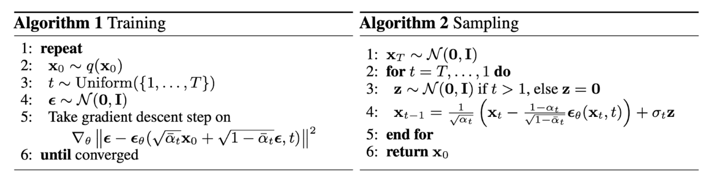
训练和采样 最终可以给出 DDPM 的训练阶段和采样(生成)/推理阶段的算法流程:
其中,Sampling 的 Line 4 的推导如下:
μ θ ( x t , t ) = 1 α t ( x t − 1 − α t 1 − α ˉ t ϵ θ ( x t , t ) ) Thus x t − 1 ∼ N ( x t − 1 ; 1 α t ( x t − 1 − α t 1 − α ˉ t ϵ θ ( x t , t ) ) , σ t I ) \begin{aligned} \boldsymbol{\mu}_\theta(\mathbf{x}_t, t) &= {\frac{1}{\sqrt{\alpha_t}} \Big( \mathbf{x}_t - \frac{1 - \alpha_t}{\sqrt{1 - \bar{\alpha}_t}} \boldsymbol{\epsilon}_\theta(\mathbf{x}_t, t) \Big)} \\ \text{Thus}\quad\mathbf{x}_{t-1} &\sim \mathcal{N}\bigg(\mathbf{x}_{t-1}; \frac{1}{\sqrt{\alpha_t}} \Big( \mathbf{x}_t - \frac{1 - \alpha_t}{\sqrt{1 - \bar{\alpha}_t}} \boldsymbol{\epsilon}_\theta(\mathbf{x}_t, t) \Big), \sigma_t\mathbf I\bigg) \end{aligned} μ θ ( x t , t ) Thus x t − 1 = α t 1 ( x t − 1 − α ˉ t 1 − α t ϵ θ ( x t , t ) ) ∼ N ( x t − 1 ; α t 1 ( x t − 1 − α ˉ t 1 − α t ϵ θ ( x t , t ) ) , σ t I )
也就是这里生成x t − 1 \mathbf{x}_{t-1} x t − 1 σ t z \sigma_t\bf z σ t z 李宏毅老师 通过类比LLM和语音模型,说明随机性的加入对模型性能具有提升的效果,具体可以参考李老师的课程视频 。李老师也谈了谈 Diffusion Models 能成功的原因,可能与 Auto-regressive 中再次融入 Auto-regressive 的思想有关系。
参数设置 在 DDPM 中,分布p θ ( x t − 1 ∣ x t ) p_\theta(\mathbf{x_{t-1}|\mathbf{x}_t}) p θ ( x t − 1 ∣ x t ) Σ θ ( x t , t ) = σ t 2 I \boldsymbol{\Sigma}_\theta(\mathbf{x}_t, t) = \sigma^2_t \mathbf{I} Σ θ ( x t , t ) = σ t 2 I σ t 2 \sigma_t^2 σ t 2
β ~ t = 1 − α ˉ t − 1 1 − α ˉ t ⋅ β t \tilde{\beta}_t = \frac{1 - \bar{\alpha}_{t-1}}{1 - \bar{\alpha}_t} \cdot \beta_t β ~ t = 1 − α ˉ t 1 − α ˉ t − 1 ⋅ β t 或是直接用β t \beta_t β t 在 DDIM 中则使用σ t ( η ) 2 = η ⋅ β ~ t \sigma_t(\eta)^2=\eta\cdot\tilde{\beta}_t σ t ( η ) 2 = η ⋅ β ~ t 0 ≤ η ≤ 1 0\leq\eta\leq1 0 ≤ η ≤ 1 IDDPM(Improved Denoising Diffusion Probabilistic Models )则利用可学习的向量v \bf v v β t \beta_t β t β ~ t \tilde{\beta}_t β ~ t
Σ θ ( x t , t ) = exp ( v log β t + ( 1 − v ) log β ~ t ) \boldsymbol{\Sigma}_\theta(\mathbf{x}_t, t) = \exp(\mathbf{v} \log \beta_t + (1-\mathbf{v}) \log \tilde{\beta}_t) Σ θ ( x t , t ) = exp ( v log β t + ( 1 − v ) log β ~ t )
IDDPM 指出当方差也可学习时(原版相当于只优化了均值),DDPM的 log-likelihood 可以进一步得到改进。
在随时间(1 ≤ t ≤ T 1\leq t\leq T 1 ≤ t ≤ T β 1 = 1 0 − 4 \beta_1=10^{-4} β 1 = 1 0 − 4 β T = 0.02 \beta_T=0.02 β T = 0.02 线性 变化,与归一化图像像素值相比,它们相对较小。而 IDDPM 采用了一种基于余弦的调度策略(类比学习率):
β t = clip ( 1 − α ˉ t α ˉ t − 1 , 0.999 ) α ˉ t = f ( t ) f ( 0 ) where f ( t ) = cos ( t / T + s 1 + s ⋅ π 2 ) 2 \beta_t = \text{clip}(1-\frac{\bar{\alpha}_t}{\bar{\alpha}_{t-1}}, 0.999) \quad\bar{\alpha}_t = \frac{f(t)}{f(0)}\quad\text{where }f(t)=\cos\Big(\frac{t/T+s}{1+s}\cdot\frac{\pi}{2}\Big)^2 β t = clip ( 1 − α ˉ t − 1 α ˉ t , 0.999 ) α ˉ t = f ( 0 ) f ( t ) where f ( t ) = cos ( 1 + s t / T + s ⋅ 2 π ) 2
由于DDPM最终推导得到的损失L simple L_{\text{simple}} L simple Σ θ \boldsymbol{\Sigma}_\theta Σ θ v \bf v v L V L B L_{VLB} L V L B L hybrid = L simple + λ L VLB L_\text{hybrid} = L_\text{simple} + \lambda L_\text{VLB} L hybrid = L simple + λ L VLB λ = 0.001 \lambda=0.001 λ = 0.001
模型架构
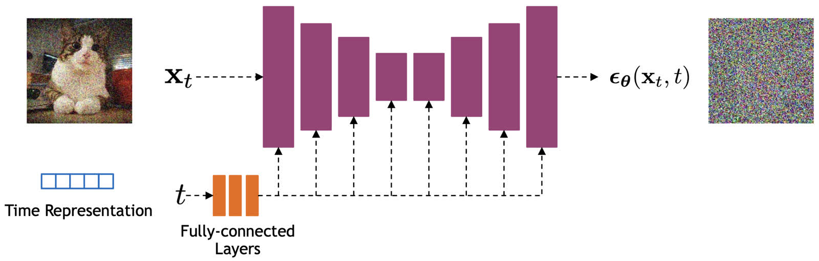
根据前面的推导可以发现,扩散模型用到神经网络的地方在于拟合噪声 ,具体来说就是接收一个噪声图 x t \mathbf x_t x t t t t ϵ θ ( x t , t ) \boldsymbol{\epsilon}_\theta(\mathbf{x}_t, t) ϵ θ ( x t , t )
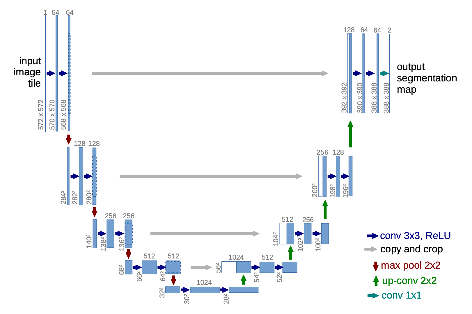
DDPM 用于预测噪声所使用的骨干网络主要是 U-Net 。值得注意的是,对于时间,我们是先得到一个 Time Embedding 再将其和噪声图一起输入给 U-Net 的。这样做的理由是可以让 U-Net 根据输入变量t t t t t t T T T T T T
U-Net (Ronneberger, et al. 2015 ) 是一种CNN模型,因其架构形状类似U型而得名。它包括两个阶段,下采样(Downsampling)和上采样(Upsampling),具体设置如下:
下采样:每个步骤包含两次重复的3x3卷积操作(Unpadding),每次卷积后接 ReLU 和步长为 2 的 2×2 MaxPooling。在每个下采样步骤中,特征通道数量翻倍。 上采样:每个步骤包含特征图的上采样操作,后接2×2卷积,每次操作将特征通道数量减半。 跳接:通过将下采样每阶段得到的特征图拼接到对应的上采样阶段的特征图上,为上采样过程提供关键的高分辨率的特征。 加速采样 (DDIM) DDPM的高质量生成依赖于较大的T T T T T T
For example, it takes around 20 hours to sample 50k images of size 32 × 32 from a DDPM, but less than a minute to do so from a GAN on an Nvidia 2080 Ti GPU.
直接将T T T x t = α t x t − 1 + 1 − α t ϵ t − 1 \mathbf x_t=\sqrt{\alpha_t} \mathbf{x}_{t-1}+\sqrt{1-\alpha_t}\boldsymbol{\epsilon}_{t-1} x t = α t x t − 1 + 1 − α t ϵ t − 1 α t \alpha_t α t 微小 噪声时保留大体 原分布。最终还有x T = α ˉ T x 0 + 1 − α ˉ T ϵ \mathbf{x}_T = \sqrt{\bar{\alpha}_T}\mathbf{x}_0 + \sqrt{1 - \bar{\alpha}_T}\boldsymbol{\epsilon} x T = α ˉ T x 0 + 1 − α ˉ T ϵ x T \mathbf{x}_T x T α ˉ t = ∏ i = 1 T α i \bar{\alpha}_t = \prod_{i=1}^T \alpha_i α ˉ t = ∏ i = 1 T α i a i a_i a i 同时 还想要它们的乘积接近0,唯一的方法只有T T T 足够大 。
加噪时能否跳步而不是一步步来?No.根源 是拟合反向的分布q ( x t − 1 ∣ x t , x 0 ) q(\mathbf{x}_{t-1} \vert \mathbf{x}_t, \mathbf{x}_0) q ( x t − 1 ∣ x t , x 0 ) 贝叶斯公式 结合q ( x t ∣ x t − 1 ) q(\mathbf{x}_t \vert \mathbf{x}_{t-1}) q ( x t ∣ x t − 1 ) 马尔可夫链 的假设。如果跳步便违反了这一假设。
DDIM(Denoising Diffusion Implicit Models )给出了一种解决方法来破解“不能跳步”的问题——干脆直接找一种不依赖于马尔可夫的(Non-Markovian)推导方法。
思路分析 在苏剑林老师的博客中给了一个很清晰的路线来归纳 DDPM 的推导:
q ( x t ∣ x t − 1 ) → 推导 q ( x t ∣ x 0 ) → 推导 q ( x t − 1 ∣ x t , x 0 ) → 近似 p θ ( x t − 1 ∣ x t ) q(\mathbf{x}_t|\mathbf{x}_{t-1})\xrightarrow{\text{推导}}q(\mathbf{x}_t|\mathbf{x}_0)\xrightarrow{\text{推导}}q(\mathbf{x}_{t-1}|\mathbf{x}_t, \mathbf{x}_0)\xrightarrow{\text{近似}}p_\theta(\mathbf{x}_{t-1}|\mathbf{x}_t) q ( x t ∣ x t − 1 ) 推导 q ( x t ∣ x 0 ) 推导 q ( x t − 1 ∣ x t , x 0 ) 近似 p θ ( x t − 1 ∣ x t )
此外,还可以总结出如下规律:
损失函数只依赖于q ( x t ∣ x 0 ) q(\mathbf{x}_t|\mathbf{x}_0) q ( x t ∣ x 0 ) 采样过程只依赖于p ( x t − 1 ∣ x t ) p(\mathbf{x}_{t-1}|\mathbf{x}_t) p ( x t − 1 ∣ x t ) 也就是说,优化目标的推导结果来看,它和依赖马尔可夫假设的q ( x t ∣ x t − 1 ) q(\mathbf{x}_t|\mathbf{x}_{t-1}) q ( x t ∣ x t − 1 ) q ( x t ∣ x t − 1 ) q(\mathbf{x}_t|\mathbf{x}_{t-1}) q ( x t ∣ x t − 1 ) q ( x t − 1 ∣ x t , x 0 ) q\left(\mathbf{x}_{t-1} \vert \mathbf{x}_t, \mathbf{x}_0\right) q ( x t − 1 ∣ x t , x 0 )
在 DDPM 中我们曾经假设过它服从于正态分布:
q ( x t − 1 ∣ x t , x 0 ) = N ( x t − 1 ; μ ~ t ( x t , x 0 ) , β ~ t I ) where μ ~ t ( x t , x 0 ) : = α ˉ t − 1 β t 1 − α ˉ t x 0 + α t ( 1 − α ˉ t − 1 ) 1 − α ˉ t x t and β ~ t : = 1 − α ˉ t − 1 1 − α ˉ t β t \begin{aligned} q\left(\mathbf{x}_{t-1} \vert \mathbf{x}_t, \mathbf{x}_0\right) & =\mathcal{N}\left(\mathbf{x}_{t-1} ; \tilde{\boldsymbol{\mu}}_t\left(\mathbf{x}_t, \mathbf{x}_0\right), \tilde{\beta}_t \mathbf{I}\right) \\ \text { where } \quad \tilde{\boldsymbol{\mu}}_t\left(\mathbf{x}_t, \mathbf{x}_0\right) & :=\frac{\sqrt{\bar{\alpha}_{t-1}} \beta_t}{1-\bar{\alpha}_t} \mathbf{x}_0+\frac{\sqrt{\alpha_t}\left(1-\bar{\alpha}_{t-1}\right)}{1-\bar{\alpha}_t} \mathbf{x}_t \quad \text { and } \quad \tilde{\beta}_t:=\frac{1-\bar{\alpha}_{t-1}}{1-\bar{\alpha}_t} \beta_t \end{aligned} q ( x t − 1 ∣ x t , x 0 ) where μ ~ t ( x t , x 0 ) = N ( x t − 1 ; μ ~ t ( x t , x 0 ) , β ~ t I ) := 1 − α ˉ t α ˉ t − 1 β t x 0 + 1 − α ˉ t α t ( 1 − α ˉ t − 1 ) x t and β ~ t := 1 − α ˉ t 1 − α ˉ t − 1 β t
既然如此我们不如直接使用待定系数法 把它定出来:
q ( x t − 1 ∣ x t , x 0 ) = N ( x t − 1 ; κ t x t + λ t x 0 , σ t 2 I ) q\left(\mathbf{x}_{t-1} \vert \mathbf{x}_t, \mathbf{x}_0\right) = \mathcal{N}(\mathbf{x}_{t-1}; \kappa_t \mathbf{x}_t + \lambda_t \mathbf{x}_0, \sigma_t^2 \mathbf{I}) q ( x t − 1 ∣ x t , x 0 ) = N ( x t − 1 ; κ t x t + λ t x 0 , σ t 2 I )
其中,约束q ( x t ∣ x 0 ) = N ( x t ; α ˉ t x 0 , ( 1 − α ˉ t ) I ) q(\mathbf{x}_t \vert \mathbf{x}_0) = \mathcal{N}(\mathbf{x}_t; \sqrt{\bar{\alpha}_t} \mathbf{x}_0, (1 - \bar{\alpha}_t)\mathbf{I}) q ( x t ∣ x 0 ) = N ( x t ; α ˉ t x 0 , ( 1 − α ˉ t ) I )
∫ q ( x t − 1 ∣ x t , x 0 ) q ( x t ∣ x 0 ) d x t = q ( x t − 1 ∣ x 0 ) \int q(\mathbf{x}_{t-1}|\mathbf{x}_t, \mathbf{x}_0) q(\mathbf{x}_t|\mathbf{x}_0)\;\mathrm d\mathbf{x}_t = q(\mathbf{x}_{t-1}|\mathbf{x}_0) ∫ q ( x t − 1 ∣ x t , x 0 ) q ( x t ∣ x 0 ) d x t = q ( x t − 1 ∣ x 0 )
事实上,满足这个边缘分布条件从采样的视角来看只需要联立下面的方程即可。
{ x t = α ˉ t x 0 + 1 − α ˉ t ϵ t ′ x t − 1 = α ˉ t − 1 x 0 + 1 − α ˉ t − 1 ϵ t − 1 ′ x t − 1 = ( κ t x t + λ t x 0 ) + σ t ϵ ′ , where ϵ t ′ , ϵ t − 1 ′ , ϵ ′ ∼ N ( 0 , I ) \begin{cases} \mathbf{x}_t &= \sqrt{\bar{\alpha}_t}\mathbf{x}_0 + \sqrt{1 - \bar{\alpha}_t}\boldsymbol{\epsilon}_t'\\ \mathbf{x}_{t-1} &= \sqrt{\bar{\alpha}_{t-1}}\mathbf{x}_0 + \sqrt{1 - \bar{\alpha}_{t-1}}\boldsymbol{\epsilon}_{t-1}'\\ \mathbf{x}_{t-1} &= (\kappa_t \mathbf{x}_t + \lambda_t \mathbf{x}_0)+{\sigma}_{t}\boldsymbol{\epsilon}'\\ \end{cases} \quad\text{, where } \boldsymbol{\epsilon}_t',\boldsymbol{\epsilon}_{t-1}',\boldsymbol{\epsilon}'\sim\mathcal{N}(\mathbf 0,\mathbf I) ⎩ ⎨ ⎧ x t x t − 1 x t − 1 = α ˉ t x 0 + 1 − α ˉ t ϵ t ′ = α ˉ t − 1 x 0 + 1 − α ˉ t − 1 ϵ t − 1 ′ = ( κ t x t + λ t x 0 ) + σ t ϵ ′ , where ϵ t ′ , ϵ t − 1 ′ , ϵ ′ ∼ N ( 0 , I )
推导如下:
x t − 1 = κ t x t + λ t x 0 + σ t ϵ ′ = κ t ( α ˉ t x 0 + 1 − α ˉ t ϵ t ′ ) + λ t x 0 + σ t ϵ ′ = ( κ t α ˉ t + λ t ) x 0 + ( κ t 1 − α ˉ t ϵ t ′ + σ t ϵ ′ ) = ( κ t α ˉ t + λ t ) x 0 + κ t 2 ( 1 − α ˉ t ) + σ t 2 ϵ x t − 1 = α ˉ t − 1 x 0 + 1 − α ˉ t − 1 ϵ t − 1 ′ \begin{aligned}\mathbf{x}_{t-1} =&\, \kappa_t \mathbf{x}_t + \lambda_t \mathbf{x}_0 + \sigma_t \boldsymbol{\epsilon}' \\ =&\, \kappa_t (\sqrt{\bar{\alpha}_t}\mathbf{x}_0 + \sqrt{1 - \bar{\alpha}_t}\boldsymbol{\epsilon}_t') + \lambda_t \boldsymbol{x}_0 + \sigma_t \boldsymbol{\epsilon}' \\ =&\, (\kappa_t \sqrt{\bar{\alpha}_t} + \lambda_t) \boldsymbol{x}_0 + (\kappa_t\sqrt{1 - \bar{\alpha}_t} \boldsymbol{\epsilon}_t' + \sigma_t \boldsymbol{\epsilon}') \\ =&\, (\kappa_t \sqrt{\bar{\alpha}_t} + \lambda_t) \boldsymbol{x}_0 + \sqrt{\kappa_t^2(1 - \bar{\alpha}_t) + \sigma_t^2}\boldsymbol{\epsilon}\\ \mathbf{x}_{t-1} =& \sqrt{\bar{\alpha}_{t-1}}\mathbf{x}_0 + \sqrt{1 - \bar{\alpha}_{t-1}}\boldsymbol{\epsilon}_{t-1}'\\ \end{aligned} x t − 1 = = = = x t − 1 = κ t x t + λ t x 0 + σ t ϵ ′ κ t ( α ˉ t x 0 + 1 − α ˉ t ϵ t ′ ) + λ t x 0 + σ t ϵ ′ ( κ t α ˉ t + λ t ) x 0 + ( κ t 1 − α ˉ t ϵ t ′ + σ t ϵ ′ ) ( κ t α ˉ t + λ t ) x 0 + κ t 2 ( 1 − α ˉ t ) + σ t 2 ϵ α ˉ t − 1 x 0 + 1 − α ˉ t − 1 ϵ t − 1 ′
对应系数相等可以得到三元一次方程组:
{ λ t + κ t α ˉ t = α ˉ t − 1 κ t 2 ( 1 − α ˉ t ) + σ t 2 = 1 − α ˉ t − 1 ⇒ ( λ t ∗ κ t ∗ σ t ∗ ) = ( α ˉ t − 1 − α ˉ t 1 − α ˉ t − 1 − σ t 2 1 − α ˉ t 1 − α ˉ t − 1 − σ t 2 1 − α ˉ t σ t ) \begin{cases} \lambda_t + \kappa_t\sqrt{\bar{\alpha}_t} = \sqrt{\bar{\alpha}_{t-1}} \\ \kappa_t^2(1 - \bar{\alpha}_t) + \sigma_t^2 = 1 - \bar{\alpha}_{t-1} \end{cases} \Rightarrow \begin{pmatrix} \lambda_t^* \\ \kappa_t^* \\ \sigma_t^* \end{pmatrix} = \begin{pmatrix} \sqrt{\bar{\alpha}_{t-1}} - \sqrt{\bar{\alpha}_t}\sqrt{\frac{1-\bar{\alpha}_{t-1}-\sigma_t^2}{1-\bar{\alpha}_t}} \\ \sqrt{\frac{1-\bar{\alpha}_{t-1}-\sigma_t^2}{1-\bar{\alpha}_t}} \\ \sigma_t \end{pmatrix} { λ t + κ t α ˉ t = α ˉ t − 1 κ t 2 ( 1 − α ˉ t ) + σ t 2 = 1 − α ˉ t − 1 ⇒ λ t ∗ κ t ∗ σ t ∗ = α ˉ t − 1 − α ˉ t 1 − α ˉ t 1 − α ˉ t − 1 − σ t 2 1 − α ˉ t 1 − α ˉ t − 1 − σ t 2 σ t
三个未知数两个方程最终会有一个自由变量,这里我们取σ t \sigma_t σ t
q ( x t − 1 ∣ x t , x 0 ) = N ( x t − 1 ; ( α ˉ t − 1 − α ˉ t 1 − α ˉ t − 1 − σ t 2 1 − α ˉ t ) x 0 + ( 1 − α ˉ t − 1 1 − α ˉ t ) x t , σ t 2 I ) = N ( x t − 1 ; α ˉ t − 1 x 0 + 1 − α ˉ t − 1 − σ t 2 x t − α ˉ t x 0 1 − α ˉ t , σ t 2 I ) \begin{aligned} q(\mathbf{x}_{t-1}|\mathbf{x}_t, \mathbf{x}_0) &= \mathcal{N}\left(\mathbf{x}_{t-1}; \left(\sqrt{\bar{\alpha}_{t-1}} - \sqrt{\bar{\alpha}_t}\sqrt{\frac{1-\bar{\alpha}_{t-1}-\sigma_t^2}{1-\bar{\alpha}_t}}\right)\mathbf{x}_0 + \left(\sqrt{\frac{1-\bar{\alpha}_{t-1}}{1-\bar{\alpha}_t}}\right)\mathbf{x}_t, \sigma_t^2\mathbf{I}\right) \\ &=\mathcal{N}\left(\mathbf{x}_{t-1}; \sqrt{\bar{\alpha}_{t-1}}\mathbf{x}_0 + \sqrt{1-\bar{\alpha}_{t-1}-\sigma_t^2}\frac{\mathbf{x}_t - \sqrt{\bar{\alpha}_t}\mathbf{x}_0}{\sqrt{1-\bar{\alpha}_t}}, \sigma_t^2\mathbf{I}\right) \end{aligned} q ( x t − 1 ∣ x t , x 0 ) = N x t − 1 ; α ˉ t − 1 − α ˉ t 1 − α ˉ t 1 − α ˉ t − 1 − σ t 2 x 0 + ( 1 − α ˉ t 1 − α ˉ t − 1 ) x t , σ t 2 I = N ( x t − 1 ; α ˉ t − 1 x 0 + 1 − α ˉ t − 1 − σ t 2 1 − α ˉ t x t − α ˉ t x 0 , σ t 2 I )
当σ t 2 \sigma_t^2 σ t 2 η \eta η σ t ( η ) 2 = η ⋅ β ~ t \sigma_t(\eta)^2=\eta\cdot\tilde{\beta}_t σ t ( η ) 2 = η ⋅ β ~ t η = 1 \eta=1 η = 1 η = 0 \eta=0 η = 0
作者针对其取值做了实验,最终得出取0时的效果最优,所以取0的版本才被正式冠以 denoising diffusion implicit model(DDIM )之名。
由于 DDIM 只在对采样q ( x t − 1 ∣ x t , x 0 ) q\left(\mathbf{x}_{t-1} \vert \mathbf{x}_t, \mathbf{x}_0\right) q ( x t − 1 ∣ x t , x 0 )
加速策略 由于DDIM抛去了马尔可夫链假设,所以加速的思路也就很简单了,跳步策略直接成为了可行方案。设τ = [ τ 1 , τ 2 , … , τ dim ( τ ) ] \boldsymbol{\tau} = [\tau_1,\tau_2,\dots,\tau_{\dim(\boldsymbol{\tau})}] τ = [ τ 1 , τ 2 , … , τ d i m ( τ ) ] [ 1 , 2 , ⋯ , T ] [1,2,\cdots,T] [ 1 , 2 , ⋯ , T ] 任意子序列 ,我们可以用α ˉ τ 1 , α ˉ τ 2 , ⋯ , α ˉ dim ( τ ) \bar{\alpha}_{\tau_1},\bar{\alpha}_{\tau_2},\cdots,\bar{\alpha}_{\dim(\boldsymbol{\tau})} α ˉ τ 1 , α ˉ τ 2 , ⋯ , α ˉ d i m ( τ ) dim ( τ ) \text{dim}(\tau) dim ( τ ) T T T
没了马尔可夫限制,采样时我们有:
q σ , s < t ( x s ∣ x t , x 0 ) = N ( x s ; α ˉ s ( x t − 1 − α ˉ t ϵ θ ( t ) ( x t ) α ˉ t ) + 1 − α ˉ s − σ t 2 ϵ θ ( t ) ( x t ) , σ t 2 I ) q_{\sigma, s < t}(\mathbf{x}_s \vert \mathbf{x}_t, \mathbf{x}_0) = \mathcal{N}(\mathbf{x}_s; \sqrt{\bar{\alpha}_s} \Big( \frac{\mathbf{x}_t - \sqrt{1 - \bar{\alpha}_t} \epsilon^{(t)}_\theta(\mathbf{x}_t)}{\sqrt{\bar{\alpha}_t}} \Big) + \sqrt{1 - \bar{\alpha}_s - \sigma_t^2} \epsilon^{(t)}_\theta(\mathbf{x}_t), \sigma_t^2 \mathbf{I}) q σ , s < t ( x s ∣ x t , x 0 ) = N ( x s ; α ˉ s ( α ˉ t x t − 1 − α ˉ t ϵ θ ( t ) ( x t ) ) + 1 − α ˉ s − σ t 2 ϵ θ ( t ) ( x t ) , σ t 2 I )
其中,ϵ θ ( t ) ( . ) \epsilon^{(t)}_\theta(.) ϵ θ ( t ) ( . ) x t \mathbf{x}_t x t x 0 \mathbf x_0 x 0 x t \mathbf x_t x t x 0 = 1 α ˉ t ( x t − 1 − α ˉ t ϵ θ ) \mathbf x_0=\frac{1}{\sqrt{\bar{\alpha}_t}}(\mathbf{x}_t - \sqrt{1 - \bar{\alpha}_t}\boldsymbol{\epsilon}_\theta) x 0 = α ˉ t 1 ( x t − 1 − α ˉ t ϵ θ )
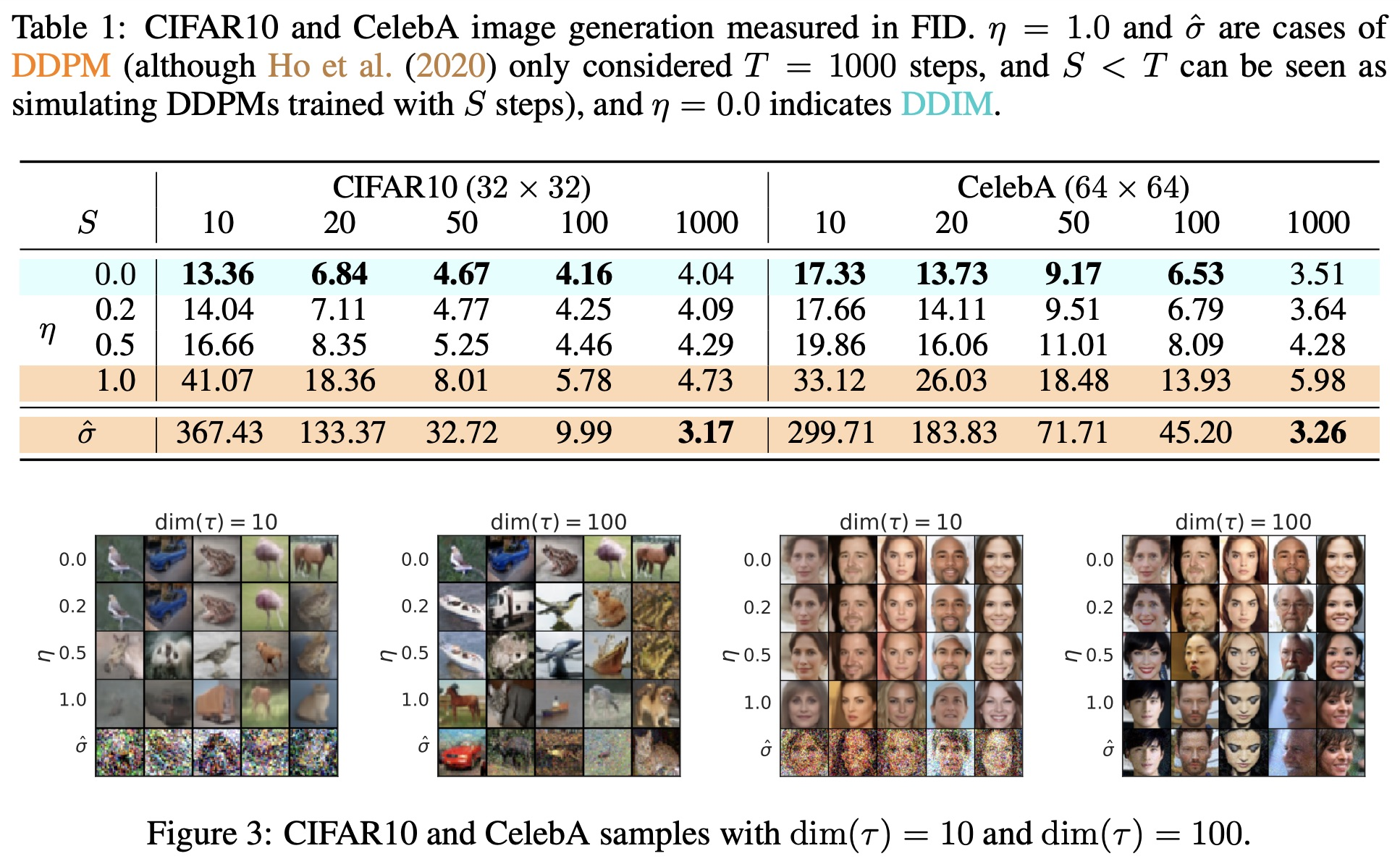
论文给出了不同的采样步长的生成效果(同样见上图)。可以看到DDIM在较小采样步长时就能达到较好的生成效果。如 CIFAR10 数据集中,S = 50 S=50 S = 50 S = 1000 S=1000 S = 1000
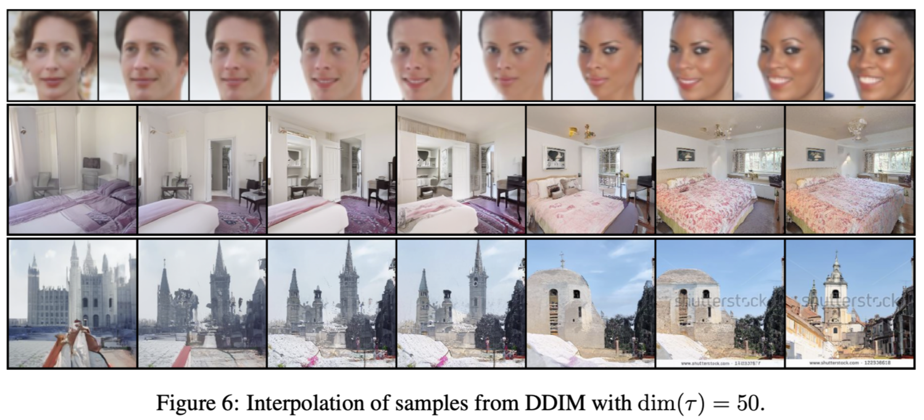
语义插值效应 因为 DDIM 将σ t \sigma_t σ t 0 0 0 x T \mathbf{x}_T x T 采样一致性 (sample consistency)。作者发现,当给定x T \mathbf{x}_T x T τ \tau τ 隐编码 信息。
有个小trick,我们在实际的生成中可以先设置较小的采样步长进行生成,若生成的图片是我们想要的,则用较大的步长重新生成高质量的图片。
即然x T \mathbf{x}_T x T
首先从高斯分布采样两个随机变量x T ( 0 ) , x T ( 1 ) \mathbf{x}_T^{(0)},\mathbf{x}_T^{(1)} x T ( 0 ) , x T ( 1 ) Slerp )对x T ( 0 ) , x T ( 1 ) \mathbf{x}_T^{(0)},\mathbf{x}_T^{(1)} x T ( 0 ) , x T ( 1 )
x T ( α ) = sin ( ( 1 − α ) θ ) sin ( θ ) x T ( 0 ) + sin ( α θ ) sin ( θ ) x T ( 1 ) \mathbf{x}_{T}^{( \alpha)}=\frac{\sin( ( 1-\alpha) \theta)} {\sin( \theta)} \mathbf{x}_{T}^{(0)}+\frac{\sin( \alpha\theta)} {\sin( \theta)} \mathbf{x}_{T}^{(1)} x T ( α ) = sin ( θ ) sin (( 1 − α ) θ ) x T ( 0 ) + sin ( θ ) sin ( α θ ) x T ( 1 )
其中θ = arccos ( ( x T ( 0 ) ) T x T ( 1 ) ∥ x T ( 0 ) ∥ ⋅ ∥ x T ( 1 ) ∥ ) \theta=\operatorname{arccos} \left( \frac{(\mathbf{x}_{T}^{(0)} )^{T} x_{T}^{(1)}} {\Vert\mathbf{x}_{T}^{(0)}\Vert\cdot \Vert\mathbf{x}_{T}^{(1)}\Vert} \right) θ = arccos ( ∥ x T ( 0 ) ∥ ⋅ ∥ x T ( 1 ) ∥ ( x T ( 0 ) ) T x T ( 1 ) )
最终发现,从左图像的生成结果插值过渡到另一个图像的过程中,图像内容会在逐渐保留其原始语义特征的情况下过渡 ,亦即 DDIM 具有语义插值效应。
和分数模型的联系 条件控制 (Condition) 作为生成模型,扩散模型跟 VAE、GAN、Flow 等模型的发展史很相似,都是先出来了无条件生成 ,然后有条件生成就紧接而来。无条件生成往往是为了探索效果上限,而有条件生成则更多是应用层面的内容,因为它可以实现根据我们的意愿(给定的某种条件)来控制模型输出我们想要的结果。
从方法上来看,条件控制生成的方式分两种:
Classifier-Guidance :事后修改。可以复用已训练好的无条件生成模型,在此基础上通过一个可学习的分类器控制条件生成。该方案的训练成本比较低,但是推断成本会高些,而且控制细节上通常没那么到位;Classifier-Free :事前训练。直接在扩散模型的训练过程中 就加入条件信号最终实现条件生成的目的。Classifier-Guidance Classifier-Guidance 最早出自《Diffusion Models Beat GANs on Image Synthesis》 ,最初就是用来实现按类 生成的;后来《More Control for Free! Image Synthesis with Semantic Diffusion Guidance》 推广了“Classifier ”的概念,使得它也可以按图、按文来生成。
从数学上来说, 带条件y \boldsymbol y y p ( x t − 1 ∣ x t ) p(\boldsymbol{x}_{t-1}|\boldsymbol{x}_t) p ( x t − 1 ∣ x t ) p ( x t − 1 ∣ x t , y ) p(\boldsymbol{x}_{t-1}|\boldsymbol{x}_t, \boldsymbol{y}) p ( x t − 1 ∣ x t , y ) p ( x t − 1 ∣ x t ) p(\boldsymbol{x}_{t-1}|\boldsymbol{x}_t) p ( x t − 1 ∣ x t )
p ( x t − 1 ∣ x t , y ) = p ( x t − 1 ∣ x t ) p ( y ∣ x t − 1 , x t ) p ( y ∣ x t ) p(\boldsymbol{x}_{t-1}|\boldsymbol{x}_t, \boldsymbol{y}) = \frac{p(\boldsymbol{x}_{t-1}|\boldsymbol{x}_t)p(\boldsymbol{y}|\boldsymbol{x}_{t-1}, \boldsymbol{x}_t)}{p(\boldsymbol{y}|\boldsymbol{x}_t)} p ( x t − 1 ∣ x t , y ) = p ( y ∣ x t ) p ( x t − 1 ∣ x t ) p ( y ∣ x t − 1 , x t )
又因为在前向过程(加噪过程)时x t \boldsymbol{x}_t x t x t − 1 \boldsymbol{x}_{t-1} x t − 1 y \boldsymbol{y} y p ( x t ∣ x t − 1 , y ) = p ( x t ∣ x t − 1 ) p(\boldsymbol{x}_{t}|\boldsymbol{x}_{t-1},\boldsymbol{y})=p(\boldsymbol{x}_{t}|\boldsymbol{x}_{t-1}) p ( x t ∣ x t − 1 , y ) = p ( x t ∣ x t − 1 )
p ( y ∣ x t − 1 , x t ) = p ( x t ∣ x t − 1 , y ) p ( y ∣ x t − 1 ) p ( x t ∣ x t − 1 ) = p ( x t ∣ x t − 1 ) p ( y ∣ x t − 1 ) p ( x t ∣ x t − 1 ) = p ( y ∣ x t − 1 ) \begin{aligned} p(\boldsymbol y|\boldsymbol x_{t-1},\boldsymbol x_{t})&=\frac{p(\boldsymbol x_{t}|\boldsymbol x_{t-1}, \boldsymbol y)p(\boldsymbol y|\boldsymbol x_{t-1})}{p(\boldsymbol x_{t}|\boldsymbol x_{t-1})}\\ &= \frac{p(\boldsymbol x_{t}|\boldsymbol x_{t-1})p(\boldsymbol y|\boldsymbol x_{t-1})}{p(\boldsymbol x_{t}|\boldsymbol x_{t-1})}\\ &= p(\boldsymbol y|\boldsymbol x_{t-1}) \end{aligned} p ( y ∣ x t − 1 , x t ) = p ( x t ∣ x t − 1 ) p ( x t ∣ x t − 1 , y ) p ( y ∣ x t − 1 ) = p ( x t ∣ x t − 1 ) p ( x t ∣ x t − 1 ) p ( y ∣ x t − 1 ) = p ( y ∣ x t − 1 )
上述等式p ( y ∣ x t − 1 , x t ) = p ( y ∣ x t − 1 ) p(\boldsymbol{y}|\boldsymbol{x}_{t-1}, \boldsymbol{x}_t)=p(\boldsymbol{y}|\boldsymbol{x}_{t-1}) p ( y ∣ x t − 1 , x t ) = p ( y ∣ x t − 1 ) x t \boldsymbol{x}_t x t x t − 1 \boldsymbol{x}_{t-1} x t − 1 ( x t − 1 , x t ) (\boldsymbol{x}_{t-1}, \boldsymbol{x}_{t}) ( x t − 1 , x t ) y \boldsymbol{y} y x t − 1 \boldsymbol{x}_{t-1} x t − 1 y \boldsymbol{y} y
最终我们需要的生成过程可调整如下:
p ( x t − 1 ∣ x t , y ) = p ( x t − 1 ∣ x t ) p ( y ∣ x t − 1 ) p ( y ∣ x t ) p(\boldsymbol{x}_{t-1}|\boldsymbol{x}_t, \boldsymbol{y}) = \frac{p(\boldsymbol{x}_{t-1}|\boldsymbol{x}_t)p(\boldsymbol{y}|\boldsymbol{x}_{t-1})}{p(\boldsymbol{y}|\boldsymbol{x}_t)} p ( x t − 1 ∣ x t , y ) = p ( y ∣ x t ) p ( x t − 1 ∣ x t ) p ( y ∣ x t − 1 )
写成log \log log
log p ( x t − 1 ∣ x t , y ) = log p ( x t − 1 ∣ x t ) + log p ( y ∣ x t − 1 ) − log p ( y ∣ x t ) \log p(\boldsymbol{x}_{t-1}|\boldsymbol{x}_t, \boldsymbol{y}) = \log p(\boldsymbol{x}_{t-1}|\boldsymbol{x}_t)+\log p(\boldsymbol{y}|\boldsymbol{x}_{t-1})-\log p(\boldsymbol{y}|\boldsymbol{x}_t) log p ( x t − 1 ∣ x t , y ) = log p ( x t − 1 ∣ x t ) + log p ( y ∣ x t − 1 ) − log p ( y ∣ x t )
考虑到当T T T x t \boldsymbol{x}_t x t x t − 1 \boldsymbol{x}_{t-1} x t − 1 泰勒展开 就有:
log p ( y ∣ x t − 1 ) − log p ( y ∣ x t ) ≈ ( x t − 1 − x t ) ⋅ ∇ x t log p ( y ∣ x t ) \log p(\boldsymbol{y}|\boldsymbol{x}_{t-1}) - \log p(\boldsymbol{y}|\boldsymbol{x}_t)\approx (\boldsymbol{x}_{t-1} - \boldsymbol{x}_t)\cdot\nabla_{\boldsymbol{x}_t} \log p(\boldsymbol{y}|\boldsymbol{x}_t) log p ( y ∣ x t − 1 ) − log p ( y ∣ x t ) ≈ ( x t − 1 − x t ) ⋅ ∇ x t log p ( y ∣ x t )
又 DDPM 中有p ( x t − 1 ∣ x t ) = N ( x t − 1 ; μ ( x t ) , σ t 2 I ) ∝ e − ∥ x t − 1 − μ ( x t ) ∥ 2 / 2 σ t 2 p(\boldsymbol{x}_{t-1}|\boldsymbol{x}_t)=\mathcal{N}(\boldsymbol{x}_{t-1};\boldsymbol{\mu}(\boldsymbol{x}_t),\sigma_t^2\mathbf{I})\propto e^{-\Vert \boldsymbol{x}_{t-1} - \boldsymbol{\mu}(\boldsymbol{x}_t)\Vert^2/2\sigma_t^2} p ( x t − 1 ∣ x t ) = N ( x t − 1 ; μ ( x t ) , σ t 2 I ) ∝ e − ∥ x t − 1 − μ ( x t ) ∥ 2 /2 σ t 2
log p ( x t − 1 ∣ x t , y ) = − 1 2 σ t 2 ∥ x t − 1 − μ ( x t ) ∥ 2 + ( x t − 1 − x t ) ∇ x t log p ( y ∣ x t ) + C 1 = − 1 2 σ t 2 ∥ x t − 1 − μ ( x t ) − σ t 2 ∇ x t log p ( y ∣ x t ) ∥ 2 + C 1 + C 2 = log p ( z ) + C \begin{aligned} \log{p(\boldsymbol x_{t-1}|\boldsymbol x_{t}, \boldsymbol y)} &= -\frac{1}{2\sigma_{t}^{2}}\|\boldsymbol x_{t-1}-\boldsymbol{\mu}(\boldsymbol x_t)\|^{2}+(\boldsymbol x_{t-1}-\boldsymbol x_{t})\nabla_{\boldsymbol x_{t}}\log{p(\boldsymbol y|\boldsymbol x_{t})}+C_{1} \\ &= -\frac{1}{2\sigma_{t}^{2}}\|\boldsymbol x_{t-1}-\boldsymbol{\mu}(\boldsymbol x_t)-\sigma_{t}^{2}\nabla_{\boldsymbol x_{t}}\log{p(\boldsymbol y|\boldsymbol x_{t})}\|^{2}+C_{1}+C_{2}\\ &= \log{p(z)}+C \end{aligned} log p ( x t − 1 ∣ x t , y ) = − 2 σ t 2 1 ∥ x t − 1 − μ ( x t ) ∥ 2 + ( x t − 1 − x t ) ∇ x t log p ( y ∣ x t ) + C 1 = − 2 σ t 2 1 ∥ x t − 1 − μ ( x t ) − σ t 2 ∇ x t log p ( y ∣ x t ) ∥ 2 + C 1 + C 2 = log p ( z ) + C
这里的C , C 1 , C 2 C,C_1,C_2 C , C 1 , C 2 x t − 1 \boldsymbol{x}_{t-1} x t − 1 无关 的式子。因为log p ( x t − 1 ∣ x t , y ) \log{p(\boldsymbol x_{t-1}|\boldsymbol x_{t}, \boldsymbol y)} log p ( x t − 1 ∣ x t , y ) x t − 1 \boldsymbol{x}_{t-1} x t − 1 f ( x t − 1 ) f(\boldsymbol{x}_{t-1}) f ( x t − 1 ) 凑出正态分布 的形状需要把部分项移动到∥ ⋅ ∥ 2 \|\cdot\|^2 ∥ ⋅ ∥ 2
如此一来,我们就可以得到p ( x t − 1 ∣ x t , y ) ∝ p ( z ) p(\boldsymbol x_{t-1}|\boldsymbol x_{t}, \boldsymbol y)\propto p(\boldsymbol{z}) p ( x t − 1 ∣ x t , y ) ∝ p ( z ) 均值 为μ ( x t ) + σ t 2 ∇ x t log p ( y ∣ x t ) \mu(\boldsymbol x_t)+\sigma_{t}^{2}\nabla_{\boldsymbol x_{t}}\log{p(\boldsymbol y|\boldsymbol x_{t})} μ ( x t ) + σ t 2 ∇ x t log p ( y ∣ x t ) σ t 2 \sigma_t^2 σ t 2
x t − 1 = μ ( x t ) + σ t 2 ∇ x t log p ( y ∣ x t ) ⏟ New Item + σ t ϵ , ϵ ∼ N ( 0 , I ) \boldsymbol{x}_{t-1} = \boldsymbol{\mu}(\boldsymbol{x}_t) {\color{skyblue}{+\underbrace{\sigma_t^2 \nabla_{\boldsymbol{x}_t} \log p(\boldsymbol{y}|\boldsymbol{x}_t)}_{\text{New Item}}}} + \sigma_t\boldsymbol{\epsilon},\quad \boldsymbol{\epsilon}\sim \mathcal{N}(\boldsymbol{0},\mathbf{I}) x t − 1 = μ ( x t ) + New Item σ t 2 ∇ x t l o g p ( y ∣ x t ) + σ t ϵ , ϵ ∼ N ( 0 , I )
与原始的扩散模型相比只需增加一项即可。
此外,原作者还指出往分类器的梯度中引入一个缩放参数γ \gamma γ
x t − 1 = μ ( x t ) + σ t 2 γ ∇ x t log p ( y ∣ x t ) + σ t ϵ , ϵ ∼ N ( 0 , I ) \boldsymbol{x}_{t-1} = \boldsymbol{\mu}(\boldsymbol{x}_t) +\sigma_t^2 {\color{skyblue}{\gamma}}\nabla_{\boldsymbol{x}_t} \log p(\boldsymbol{y}|\boldsymbol{x}_t) + \sigma_t\boldsymbol{\epsilon},\quad \boldsymbol{\epsilon}\sim \mathcal{N}(\boldsymbol{0},\mathbf{I}) x t − 1 = μ ( x t ) + σ t 2 γ ∇ x t log p ( y ∣ x t ) + σ t ϵ , ϵ ∼ N ( 0 , I )
当γ > 1 \gamma\gt1 γ > 1 γ \gamma γ
Classifier-Guidance 的推导同样还可以用 Score function 来理解,会更加清晰和直观。并且采用这种推导方式解决了σ t ≠ 0 \sigma_t\neq0 σ t = 0 σ t = 0 \sigma_t=0 σ t = 0
Classifier-Free Classifier-Free 方案本身没什么理论上的技巧,它是条件扩散模型最朴素的方案,出现得晚只是因为重新训练扩散模型的成本较大吧,在数据和算力都比较充裕的前提下,Classifier-Free方案表现出了令人惊叹的细节控制能力。
具体来说,该方案直接假设:
p ( x t − 1 ∣ x t , y ) = N ( x t − 1 ; μ ( x t , y ) , σ t 2 I ) p(\boldsymbol{x}_{t-1}|\boldsymbol{x}_t, \boldsymbol{y}) = \mathcal{N}(\boldsymbol{x}_{t-1}; \boldsymbol{\mu}(\boldsymbol{x}_t, \boldsymbol{y}),\sigma_t^2\mathbf{I}) p ( x t − 1 ∣ x t , y ) = N ( x t − 1 ; μ ( x t , y ) , σ t 2 I )
与 DDPM 类似,条件y \boldsymbol{y} y μ ( ) \boldsymbol{\mu}() μ ( ) ϵ θ ( ) \boldsymbol{\epsilon}_\theta() ϵ θ ( )
μ ( x t , y ) = 1 α t ( x t − 1 − α t 1 − α ˉ t ϵ θ ( x t , y , t ) ) \boldsymbol{\mu}(\boldsymbol{x}_t, \boldsymbol{y}) = {\frac{1}{\sqrt{\alpha_t}} \Big( \boldsymbol{x}_t - \frac{1 - \alpha_t}{\sqrt{1 - \bar{\alpha}_t}} \boldsymbol{\epsilon}_\theta(\boldsymbol{x}_t, \boldsymbol{y},t) \Big)} μ ( x t , y ) = α t 1 ( x t − 1 − α ˉ t 1 − α t ϵ θ ( x t , y , t ) )
值得一提的是,Classifier-Guidance 中的均值函数:μ ( x t ) + σ t 2 ∇ x t log p ( y ∣ x t ) \boldsymbol{\mu}(\boldsymbol x_t)+\sigma_{t}^{2}\nabla_{\boldsymbol x_{t}}\log{p(\boldsymbol y|\boldsymbol x_{t})} μ ( x t ) + σ t 2 ∇ x t log p ( y ∣ x t ) μ ( x t , y ) \boldsymbol{\mu}(\boldsymbol{x}_t, \boldsymbol{y}) μ ( x t , y )
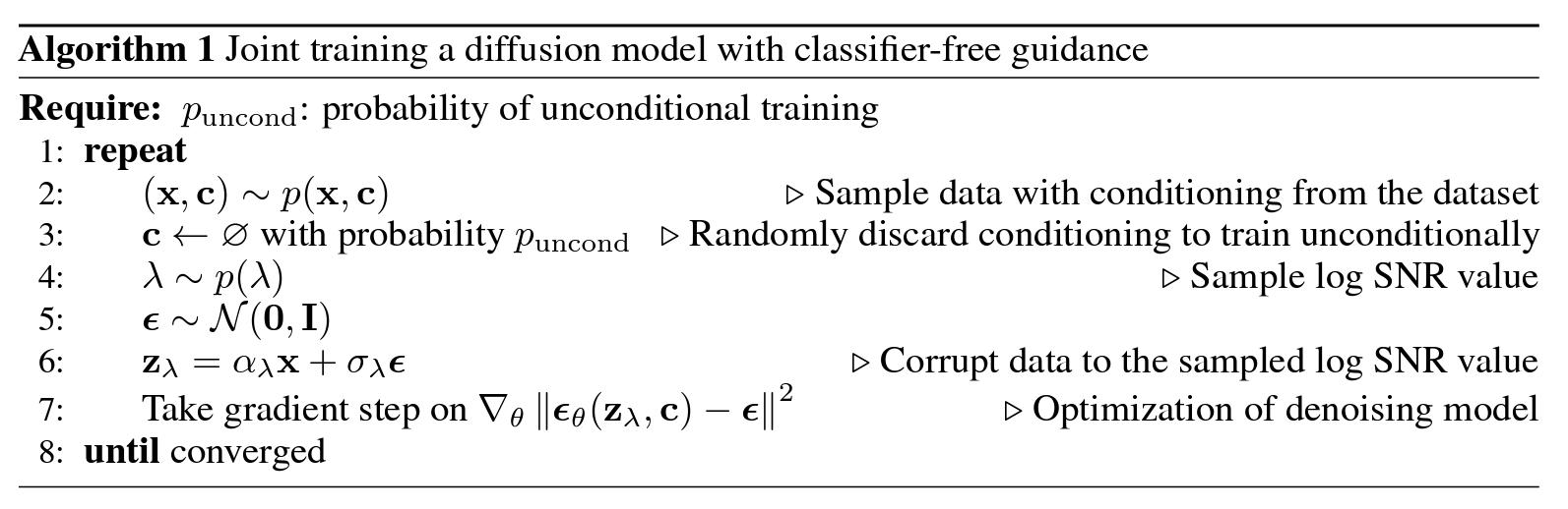
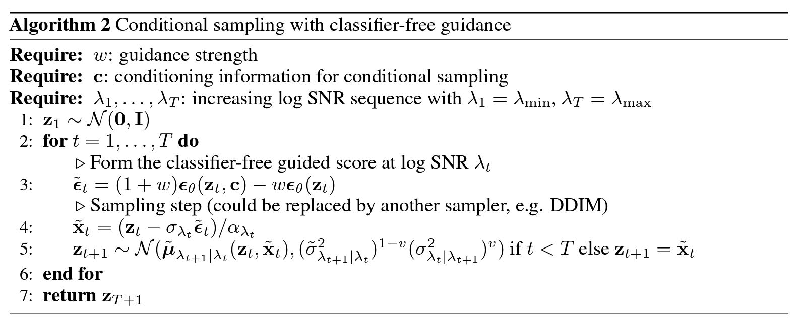
此外,Classifier-Free 也应用了缩放机制,设置一个参数λ \lambda λ 有条件生成 的部分和无条件生成 的部分组合起来。最终可以写为:
ϵ ~ θ ( x t , y , t ) = λ ϵ θ ( x t , y , t ) + ( 1 − λ ) ϵ θ ( x t , t ) \tilde{\boldsymbol{\epsilon}}_\theta(\boldsymbol{x}_t, \boldsymbol{y},t)=\lambda\boldsymbol{\epsilon}_\theta(\boldsymbol{x}_t, \boldsymbol{y},t)+(1-\lambda)\boldsymbol{\epsilon}_\theta(\boldsymbol{x}_t,t) ϵ ~ θ ( x t , y , t ) = λ ϵ θ ( x t , y , t ) + ( 1 − λ ) ϵ θ ( x t , t )
这样一来看似需要学习两种模型,但实际上要实现无条件生成,不一定要去掉额外的条件输入,直接把条件输入替换成某个固定的空值∅ \varnothing ∅ ϵ θ ( x t , y , t ) \boldsymbol{\epsilon}_\theta(\boldsymbol{x}_t, \boldsymbol{y},t) ϵ θ ( x t , y , t ) y = ∅ \boldsymbol{y}=\varnothing y = ∅ c \bf c c ∅ \varnothing ∅
下面是论文中给出的训练算法和采样算法:
Classifier-Free 的推导也可以用 Score function 来与 Classifier-Guidance 进一步联系起来,简单来说它通过一个隐式 分类器来替代Classifier-Guidance中的显式 分类器,从而无需直接计算分类器及其梯度。
潜在扩散 (LDM) 之前的扩散模型(包括DDPM、DDIM以及其他我们没有介绍到的变体)一直面临着采样空间太大,学习的噪声维度和图像的维度同样大尺寸的问题。因此利用扩散模型进行高分辨率图像生成时,需要的计算资源会急剧增加,虽然 DDIM 等工作已经对此有所改善,但效果依然有限。
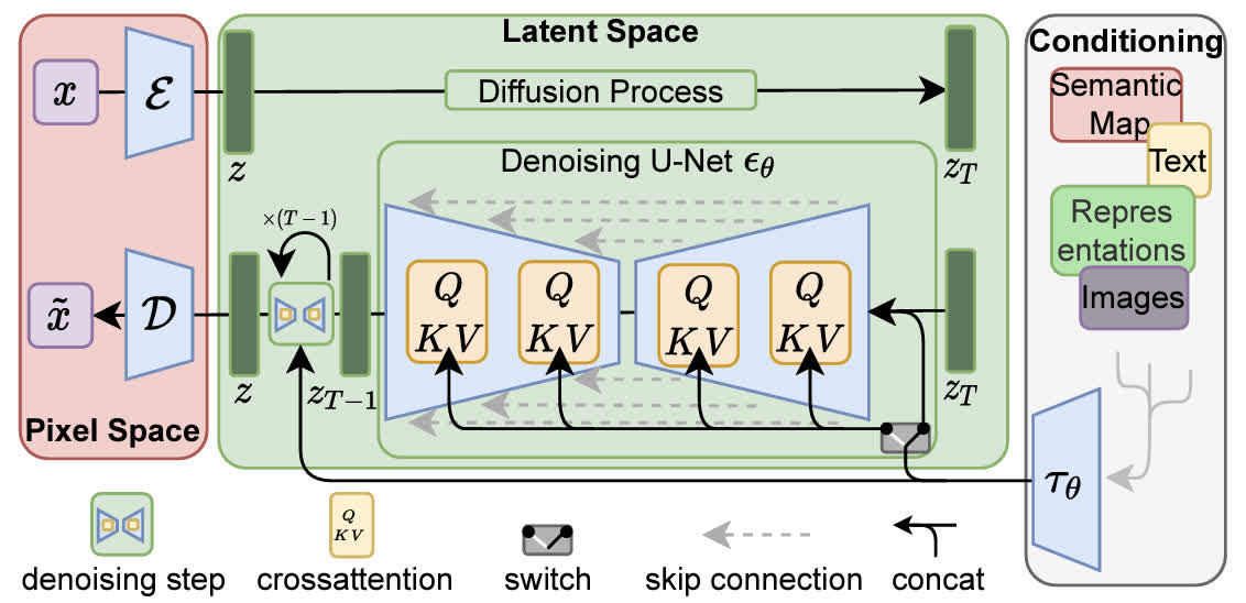
对此,LDM(Latent Diffusion Model)先使用一个预训练好的 AutoEncoder,将图片像素转换到了维度较小的 Latent Space 上,而后再进行传统的扩散模型推理与优化。这种训练方式使得 LDM 在算力和性能之间得到了平衡。
此外,通过引入交叉注意力 ,使得 DMs 能够在条件生成上有不错的效果,包括如文生图(text-to-image),图像修复(inpainting) 等。
它也是大名鼎鼎的 Stable Diffusion 的核心架构。Stable Diffusion 正是在这个通用架构的基础上进行了实现和训练得来的, 推动了生成式扩散模型在工程上的应用。
图像感知压缩 如前文所述,LDM 把图像生成过程从原始的图像像素空间转换到了一个隐空间。具体来说,对于一个维度为 x ∈ R H × W × 3 \mathbf{x}\in\mathbb{R}^{H\times W\times3} x ∈ R H × W × 3 VAE 的 encoder E \mathcal{E} E z = E ( x ) \mathbf{z}=\mathcal{E}(\mathbf{x}) z = E ( x ) D \mathcal D D x ~ = D ( E ( x ) ) \tilde{\mathbf{x}}=\mathcal{D}(\mathcal{E}(\mathbf{x})) x ~ = D ( E ( x ))
为了防止压缩后的空间是某个高方差的空间,需要进行正则化。作者给出了两种正则化方案:第一种是 KL-正则化 ,也就是将隐变量和标准高斯分布使用一个 KL 惩罚项进行正则化;第二种是 VQ-正则化 ,也就是使用一个 Vector Quantization 层进行正则化。
Encoding 涉及到下采样,作者测试了一系列下采样倍数 f ∈ { 1 , 2 , 4 , 8 , 16 , 32 } f\in\{1, 2, 4, 8, 16, 32\} f ∈ { 1 , 2 , 4 , 8 , 16 , 32 }
你可能会产生这样的疑惑:既然LDM首先就利用了VAE得到 Latent Space 的 encoding,根据VAE的思想,这个 encoding 不就天然已经服从于标准高斯分布了吗?在它的基础上继续做 Diffusion 的意义在哪里?
实际上 LDM 中对 VAE 的 KL-正则化 前面的系数因子其实是很小很小的(1e-6),换句话说 LDM 中 VAE 基本上是当做简单的 AE 来用。(相关链接:Kylin的回答 - 知乎 )
条件注入 LDM并没有在 Diffusion 的设计上做什么技术上的改进,仅仅只是将原始的优化目标调整到隐空间中。
L DM = E x , ϵ ∼ N ( 0 , 1 ) , t [ ∣ ∣ ϵ − ϵ θ ( x t , t ) ∣ ∣ 2 2 ] L LDM = E E ( x ) , ϵ ∼ N ( 0 , 1 ) , t [ ∣ ∣ ϵ − ϵ θ ( x t , t ) ∣ ∣ 2 2 ] \begin{aligned} L_\textrm{DM}&=\mathbb{E}_{\mathbf{x},\epsilon\sim\mathcal{N}(0,1),t}\left[||\epsilon-\epsilon_\theta(\mathbf{x}_t,t)||_2^2\right]\\ L_\textrm{LDM}&=\mathbb{E}_{\textcolor{red}{\mathcal{E}(\mathbf{x})},\epsilon\sim\mathcal{N}(0,1),t}\left[||\epsilon-\epsilon_\theta(\mathbf{x}_t,t)||_2^2\right] \end{aligned} L DM L LDM = E x , ϵ ∼ N ( 0 , 1 ) , t [ ∣∣ ϵ − ϵ θ ( x t , t ) ∣ ∣ 2 2 ] = E E ( x ) , ϵ ∼ N ( 0 , 1 ) , t [ ∣∣ ϵ − ϵ θ ( x t , t ) ∣ ∣ 2 2 ]
部分代码解析 此处所给代码均摘自 LDM 官方的 Pytorch 实现 CompVis/latent-diffusion
DDPM 构造函数 DDPM 类是 lightning.LightningModule 的派生类,因此继承了 cpkt_path、ignore_keys、train_step 等相关方法,由于本解析只说明关键部分,所以略去了对其的代码展示。
1
2
3
4
5
6
7
8
9
10
11
12
13
14
15
16
17
18
19
20
21
22
23
24
25
26
27
28
29
30
31
32
33
34
35
36
37
38
39
40
41
42
43
44
45
46
47
48
49
50
51
52
class DDPM (pl.LightningModule): def __init__ (self, unet_config, timesteps=1000 , beta_schedule="linear" , loss_type="l2" , clip_denoised=True , linear_start=1e-4 , linear_end=2e-2 , cosine_s=8e-3 , given_betas=None , original_elbo_weight=0. , v_posterior=0. , parameterization="eps" , l_simple_weight=1. , learn_logvar=False , logvar_init=0. , ): super ().__init__() assert parameterization in ["eps" , "x0" ], 'currently only supporting "eps" and "x0"' self.parameterization = parameterization self.clip_denoised = clip_denoised self.image_size = image_size self.channels = channels self.use_positional_encodings = use_positional_encodings self.model = DiffusionWrapper(unet_config, conditioning_key) self.v_posterior = v_posterior self.original_elbo_weight = original_elbo_weight self.l_simple_weight = l_simple_weight self.loss_type = loss_type self.register_schedule(given_betas=given_betas, beta_schedule=beta_schedule, timesteps=timesteps, linear_start=linear_start, linear_end=linear_end, cosine_s=cosine_s) self.learn_logvar = learn_logvar self.logvar = torch.full(fill_value=logvar_init, size=(self.num_timesteps,)) if self.learn_logvar: self.logvar = nn.Parameter(self.logvar, requires_grad=True )
DiffusionWarpper 其中的 DiffusionWrapper 为预测噪声的模型,通常是 UNet,为了实现带条件或不带条件以及带条件的方式,单独封装了这个类:
1
2
3
4
5
6
7
8
9
10
11
12
13
14
15
16
17
18
19
20
21
22
23
24
25
26
27
class DiffusionWrapper (pl.LightningModule): def __init__ (self, net_config, conditioning_key ): super ().__init__() self.diffusion_model = UNetModel(net_config) self.conditioning_key = conditioning_key assert self.conditioning_key in [None , 'concat' , 'crossattn' , 'hybrid' , 'adm' ] def forward (self, x, t, c_concat: list = None , c_crossattn: list = None ): if self.conditioning_key is None : out = self.diffusion_model(x, t) elif self.conditioning_key == 'concat' : xc = torch.cat([x] + c_concat, dim=1 ) out = self.diffusion_model(xc, t) elif self.conditioning_key == 'crossattn' : cc = torch.cat(c_crossattn, 1 ) out = self.diffusion_model(x, t, context=cc) elif self.conditioning_key == 'hybrid' : xc = torch.cat([x] + c_concat, dim=1 ) cc = torch.cat(c_crossattn, 1 ) out = self.diffusion_model(xc, t, context=cc) elif self.conditioning_key == 'adm' : cc = c_crossattn[0 ] out = self.diffusion_model(x, t, y=cc) else : raise NotImplementedError() return out
注册β \beta β α \alpha α 1 2 3 4 5 6 7 8 9 10 11 12 13 14 15 16 17 18 19 20 21 22 23 24 25 26 27 28 29 30 31 32 33 34 35 36 37 38 39 40 41 42 43 44 45 46 47 48 49 50 51 52 53 54 55 56 57 58 59 60 61 62 63 64 65 66 def register_schedule (self, given_betas=None , beta_schedule="linear" , timesteps=1000 , linear_start=1e-4 , linear_end=2e-2 , cosine_s=8e-3 ): if given_betas: betas = given_betas else : betas = make_beta_schedule(beta_schedule, timesteps, linear_start=linear_start, linear_end=linear_end, cosine_s=cosine_s) alphas = 1. - betas alphas_cumprod = np.cumprod(alphas, axis=0 ) alphas_cumprod_prev = np.append(1. , alphas_cumprod[:-1 ]) timesteps, = betas.shape self.num_timesteps = int (timesteps) self.linear_start = linear_start self.linear_end = linear_end assert alphas_cumprod.shape[0 ] == self.num_timesteps, 'alphas have to be defined for each timestep' to_torch = partial(torch.tensor, dtype=torch.float32) self.register_buffer('betas' , to_torch(betas)) self.register_buffer('alphas_cumprod' , to_torch(alphas_cumprod)) self.register_buffer('alphas_cumprod_prev' , to_torch(alphas_cumprod_prev)) self.register_buffer('sqrt_alphas_cumprod' , to_torch(np.sqrt(alphas_cumprod))) self.register_buffer('sqrt_one_minus_alphas_cumprod' , to_torch(np.sqrt(1. - alphas_cumprod))) self.register_buffer('log_one_minus_alphas_cumprod' , to_torch(np.log(1. - alphas_cumprod))) self.register_buffer('sqrt_recip_alphas_cumprod' , to_torch(np.sqrt(1. / alphas_cumprod))) self.register_buffer('sqrt_recipm1_alphas_cumprod' , to_torch(np.sqrt(1. / alphas_cumprod - 1 ))) posterior_variance = (1 - self.v_posterior) * betas * (1. - alphas_cumprod_prev) / (1. - alphas_cumprod) + self.v_posterior * betas self.register_buffer('posterior_variance' , to_torch(posterior_variance)) self.register_buffer('posterior_log_variance_clipped' , to_torch(np.log(np.maximum(posterior_variance, 1e-20 )))) self.register_buffer('posterior_mean_coef1' , to_torch( betas * np.sqrt(alphas_cumprod_prev) / (1. - alphas_cumprod))) self.register_buffer('posterior_mean_coef2' , to_torch( (1. - alphas_cumprod_prev) * np.sqrt(alphas) / (1. - alphas_cumprod))) if self.parameterization == "eps" : lvlb_weights = self.betas ** 2 / ( 2 * self.posterior_variance * to_torch(alphas) * (1 - self.alphas_cumprod)) elif self.parameterization == "x0" : lvlb_weights = 0.5 * np.sqrt(torch.Tensor(alphas_cumprod)) / (2. * 1 - torch.Tensor(alphas_cumprod)) else : raise NotImplementedError("mu not supported" ) lvlb_weights[0 ] = lvlb_weights[1 ] self.register_buffer('lvlb_weights' , lvlb_weights, persistent=False ) assert not torch.isnan(self.lvlb_weights).all ()
make_beta_schedule make_beta_schedule 函数定义在 DDPM Class 外,用于预先生成一组β \beta β
1 2 3 4 5 6 7 8 9 10 11 12 13 14 15 16 17 18 19 20 21 22 23 def make_beta_schedule (schedule, n_timestep, linear_start=1e-4 , linear_end=2e-2 , cosine_s=8e-3 ): if schedule == "linear" : betas = ( torch.linspace(linear_start ** 0.5 , linear_end ** 0.5 , n_timestep, dtype=torch.float64) ** 2 ) elif schedule == "cosine" : timesteps = ( torch.arange(n_timestep + 1 , dtype=torch.float64) / n_timestep + cosine_s ) alphas = timesteps / (1 + cosine_s) * np.pi / 2 alphas = torch.cos(alphas).pow (2 ) alphas = alphas / alphas[0 ] betas = 1 - alphas[1 :] / alphas[:-1 ] betas = np.clip(betas, a_min=0 , a_max=0.999 ) elif schedule == "sqrt_linear" : betas = torch.linspace(linear_start, linear_end, n_timestep, dtype=torch.float64) elif schedule == "sqrt" : betas = torch.linspace(linear_start, linear_end, n_timestep, dtype=torch.float64) ** 0.5 else : raise ValueError(f"schedule '{schedule} ' unknown." ) return betas.numpy()
前向加噪过程 计算q ( x t ∣ x 0 ) = N ( x t ; α ˉ t x 0 , ( 1 − α ˉ t ) I ) q(\mathbf{x}_t \vert \mathbf{x}_0) = \mathcal{N}(\mathbf{x}_t; \sqrt{\bar{\alpha}_t} \mathbf{x}_0, (1 - \bar{\alpha}_t)\mathbf{I}) q ( x t ∣ x 0 ) = N ( x t ; α ˉ t x 0 , ( 1 − α ˉ t ) I ) x t \mathbf x_t x t 1 2 3 4 5 6 7 8 9 10 11 12 13 14 15 16 17 def q_mean_variance (self, x_start, t ): """ Get the distribution q(x_t | x_0). :param x_start: the [N x C x ...] tensor of noiseless inputs. :param t: the number of diffusion steps (minus 1). Here, 0 means one step. :return: A tuple (mean, variance, log_variance), all of x_start's shape. """ mean = (extract_into_tensor(self.sqrt_alphas_cumprod, t, x_start.shape) * x_start) variance = extract_into_tensor(1.0 - self.alphas_cumprod, t, x_start.shape) log_variance = extract_into_tensor(self.log_one_minus_alphas_cumprod, t, x_start.shape) return mean, variance, log_variance def q_sample (self, x_start, t, noise=None ): noise = torch.randn_like(x_start) if noise is None else noise return (extract_into_tensor(self.sqrt_alphas_cumprod, t, x_start.shape) * x_start + extract_into_tensor(self.sqrt_one_minus_alphas_cumprod, t, x_start.shape) * noise)
给定噪声反过来计算x 0 = 1 α ˉ t x t − 1 α ˉ t − 1 ϵ t ( ⋆ ) \mathbf{x}_0=\sqrt{\frac1{\bar{\alpha}_t}}\;\mathbf{x}_t-\sqrt{\frac1{\bar{\alpha}_t}-1}\;\boldsymbol{\epsilon}_t\quad(\star) x 0 = α ˉ t 1 x t − α ˉ t 1 − 1 ϵ t ( ⋆ ) 1 2 3 4 5 def predict_start_from_noise (self, x_t, t, noise ): return ( extract_into_tensor(self.sqrt_recip_alphas_cumprod, t, x_t.shape) * x_t - extract_into_tensor(self.sqrt_recipm1_alphas_cumprod, t, x_t.shape) * noise )
计算带x 0 \mathbf x_0 x 0 q ( x t − 1 ∣ x t , x 0 ) q(\mathbf{x}_{t-1} \vert \mathbf{x}_t, \mathbf{x}_0) q ( x t − 1 ∣ x t , x 0 ) 1 2 3 4 5 6 7 8 def q_posterior (self, x_start, x_t, t ): posterior_mean = ( extract_into_tensor(self.posterior_mean_coef1, t, x_t.shape) * x_start + extract_into_tensor(self.posterior_mean_coef2, t, x_t.shape) * x_t ) posterior_variance = extract_into_tensor(self.posterior_variance, t, x_t.shape) posterior_log_variance_clipped = extract_into_tensor(self.posterior_log_variance_clipped, t, x_t.shape) return posterior_mean, posterior_variance, posterior_log_variance_clipped
extract_into_tensor 其中函数 extract_into_tensor(a, t, x_shape) 定义在 Class 外,表示从数组 a 中拿取第 t 个元素, 并 reshape 为兼容 x_shape 的形状的 torch.tensor 对象.
1 2 3 4 def extract_into_tensor (a, t, x_shape ): b, *_ = t.shape out = a.gather(-1 , t) return out.reshape(b, *((1 ,) * (len (x_shape) - 1 )))
反向去噪过程 将 (★) 式中的ϵ t \boldsymbol\epsilon_t ϵ t self.model)预测,然后代入到条件后验分布q ( x t − 1 ∣ x t , x 0 ) q(\mathbf{x}_{t-1} \vert \mathbf{x}_t, \mathbf{x}_0) q ( x t − 1 ∣ x t , x 0 ) self.q_posterior)中,得到p θ ( x t − 1 ∣ x t ) p_\theta(\mathbf{x}_{t-1} \vert \mathbf{x}_t) p θ ( x t − 1 ∣ x t ) 1 2 3 4 5 6 7 8 9 10 11 def p_mean_variance (self, x, t, clip_denoised: bool ): model_out = self.model(x, t) if self.parameterization == "eps" : x_recon = self.predict_start_from_noise(x, t=t, noise=model_out) elif self.parameterization == "x0" : x_recon = model_out if clip_denoised: x_recon.clamp_(-1. , 1. ) model_mean, posterior_variance, posterior_log_variance = self.q_posterior(x_start=x_recon, x_t=x, t=t) return model_mean, posterior_variance, posterior_log_variance
1 2 3 4 5 6 7 8 9 10 11 12 13 14 15 16 17 18 19 20 21 22 23 24 25 26 27 28 29 30 31 32 33 34 @torch.no_grad() def p_sample (self, x, t, clip_denoised=True , repeat_noise=False ): b, *_, device = *x.shape, x.device model_mean, _, model_log_variance = self.p_mean_variance(x=x, t=t, clip_denoised=clip_denoised) noise = noise_like(x.shape, device, repeat_noise) nonzero_mask = (1 - (t == 0 ).float ()).reshape(b, *((1 ,) * (len (x.shape) - 1 ))) return model_mean + nonzero_mask * (0.5 * model_log_variance).exp() * noise @torch.no_grad() def p_sample_loop (self, shape, return_intermediates=False ): device = self.betas.device b = shape[0 ] img = torch.randn(shape, device=device) intermediates = [img] for i in tqdm(reversed (range (0 , self.num_timesteps)), desc='Sampling t' , total=self.num_timesteps): img = self.p_sample(img, torch.full((b,), i, device=device, dtype=torch.long), clip_denoised=self.clip_denoised) if i % self.log_every_t == 0 or i == self.num_timesteps - 1 : intermediates.append(img) if return_intermediates: return img, intermediates return img @torch.no_grad() def sample (self, batch_size=16 , return_intermediates=False ): image_size = self.image_size channels = self.channels return self.p_sample_loop((batch_size, channels, image_size, image_size), return_intermediates=return_intermediates)
noise_like 其中函数 noise_like(shape, device, repeat=False) 定义在 Class 外,返回一个和 x 一样形状的标准高斯噪音 noise:
1 2 3 4 def noise_like (shape, device, repeat=False ): repeat_noise = lambda : torch.randn((1 , *shape[1 :]), device=device).repeat(shape[0 ], *((1 ,) * (len (shape) - 1 ))) noise = lambda : torch.randn(shape, device=device) return repeat_noise() if repeat else noise()
损失函数计算 给定时间步t t t ϵ t \boldsymbol\epsilon_t ϵ t x 0 \mathbf x_0 x 0 x t \mathbf x_t x t self.q_sample),然后输入x t \mathbf x_t x t t t t c c c self.model)预测噪声ϵ θ \boldsymbol\epsilon_\theta ϵ θ model_out)。然后计算噪声之间的直接损失(self.get_loss),根据参数调整这个直接的 Simple Loss 和 VLB Loss 的比重。
1 2 3 4 5 6 7 8 9 10 11 12 13 14 15 16 17 18 19 20 21 22 23 24 25 26 27 28 29 30 31 32 33 34 35 36 37 38 39 40 41 42 43 44 45 46 47 48 49 def get_loss (self, pred, target, mean=True ): if self.loss_type == 'l1' : loss = (target - pred).abs () if mean: loss = loss.mean() elif self.loss_type == 'l2' : if mean: loss = torch.nn.functional.mse_loss(target, pred) else : loss = torch.nn.functional.mse_loss(target, pred, reduction='none' ) else : raise NotImplementedError("unknown loss type '{loss_type}'" ) return loss def p_losses (self, x_start, t, noise=None ): noise = torch.randn_like(x_start) if noise is None else noise x_noisy = self.q_sample(x_start=x_start, t=t, noise=noise) model_out = self.model(x_noisy, t) loss_dict = {} if self.parameterization == "eps" : target = noise elif self.parameterization == "x0" : target = x_start else : raise NotImplementedError(f"Paramterization {self.parameterization} not yet supported" ) loss = self.get_loss(model_out, target, mean=False ).mean(dim=[1 , 2 , 3 ]) log_prefix = 'train' if self.training else 'val' loss_dict.update({f'{log_prefix} /loss_simple' : loss.mean()}) loss_simple = loss.mean() * self.l_simple_weight loss_vlb = (self.lvlb_weights[t] * loss).mean() loss_dict.update({f'{log_prefix} /loss_vlb' : loss_vlb}) loss = loss_simple + self.original_elbo_weight * loss_vlb loss_dict.update({f'{log_prefix} /loss' : loss}) return loss, loss_dict def forward (self, x, *args, **kwargs ): t = torch.randint(0 , self.num_timesteps, (x.shape[0 ],), device=self.device).long() return self.p_losses(x, t, *args, **kwargs)
训练验证步 1 2 3 4 5 6 7 8 9 10 11 12 13 14 15 16 17 18 19 20 21 22 23 24 25 26 27 28 29 30 31 32 33 34 35 36 37 38 39 40 41 def get_input (self, batch ): x = batch if len (x.shape) == 3 : x = x[..., None ] x = rearrange(x, 'b h w c -> b c h w' ) x = x.to(memory_format=torch.contiguous_format).float () return x def shared_step (self, batch ): x = self.get_input(batch) loss, loss_dict = self(x) return loss, loss_dict def training_step (self, batch, batch_idx ): loss, loss_dict = self.shared_step(batch) self.log_dict(loss_dict, prog_bar=True , logger=True , on_step=True , on_epoch=True ) self.log("global_step" , self.global_step, prog_bar=True , logger=True , on_step=True , on_epoch=False ) if self.use_scheduler: lr = self.optimizers().param_groups[0 ]['lr' ] self.log('lr_abs' , lr, prog_bar=True , logger=True , on_step=True , on_epoch=False ) return loss @torch.no_grad() def validation_step (self, batch, batch_idx ): _, loss_dict_no_ema = self.shared_step(batch) self.log_dict(loss_dict_no_ema, prog_bar=False , logger=True , on_step=False , on_epoch=True ) def configure_optimizers (self ): lr = self.learning_rate params = list (self.model.parameters()) if self.learn_logvar: params = params + [self.logvar] opt = torch.optim.AdamW(params, lr=lr) return opt
条件生成 构造函数 CondDiffusion 继承 DDPM 类,扩充实现了条件生成部分1 2 3 4 5 6 7 8 9 10 11 12 13 14 15 16 17 18 19 20 21 22 23 24 25 26 27 28 29 30 31 32 33 34 35 36 37 38 39 40 41 class CondDiffusion (DDPM ): def __init__ (self, first_stage_model, cond_stage_model, num_timesteps_cond=None , cond_stage_trainable=False , concat_mode=True , conditioning_key=None , *args, **kwargs ): self.num_timesteps_cond = num_timesteps_cond if num_timesteps_cond is not None else 1 assert self.num_timesteps_cond <= kwargs['timesteps' ] if conditioning_key is None : conditioning_key = 'concat' if concat_mode else 'crossattn' ckpt_path = kwargs.pop("ckpt_path" , None ) ignore_keys = kwargs.pop("ignore_keys" , []) super ().__init__(conditioning_key=conditioning_key, *args, **kwargs) if cond_stage_trainable: self.cond_stage_model = cond_stage_model.train() else : self.cond_stage_model = cond_stage_model.eval () for param in self.first_stage_model.parameters(): param.requires_grad = False self.first_stage_model = first_stage_model.eval () for param in self.first_stage_model.parameters(): param.requires_grad = False self.restarted_from_ckpt = False if ckpt_path is not None : self.init_from_ckpt(ckpt_path, ignore_keys) self.restarted_from_ckpt = True
注册条件时间表 1 2 3 4 5 6 7 8 9 10 11 12 13 14 15 def make_cond_schedule (self, ): self.cond_ids = torch.full(size=(self.num_timesteps,), fill_value=self.num_timesteps - 1 , dtype=torch.long) ids = torch.round (torch.linspace(0 , self.num_timesteps - 1 , self.num_timesteps_cond)).long() self.cond_ids[:self.num_timesteps_cond] = ids def register_schedule (self, given_betas=None , beta_schedule="linear" , timesteps=1000 , linear_start=1e-4 , linear_end=2e-2 , cosine_s=8e-3 ): super ().register_schedule(given_betas, beta_schedule, timesteps, linear_start, linear_end, cosine_s) self.shorten_cond_schedule = self.num_timesteps_cond > 1 if self.shorten_cond_schedule: self.make_cond_schedule()
训练步重构 1 2 3 4 5 6 7 8 9 10 11 12 13 14 15 16 17 18 19 20 21 22 23 24 25 26 27 28 29 30 31 32 33 34 35 36 37 38 39 40 41 42 43 44 45 46 47 48 49 50 51 52 53 54 55 56 57 58 59 60 61 62 63 64 65 66 def shared_step (self, batch, **kwargs ): x, c = batch x = self.encode_first_stage(x) c = self.encode_cond_stage(c) loss = self(x, c) return loss def forward (self, x, c, *args, **kwargs ): t = torch.randint(0 , self.num_timesteps, (x.shape[0 ],), device=self.device).long() if self.model.conditioning_key is not None : assert c is not None if self.shorten_cond_schedule: tc = self.cond_ids[t].to(self.device) c = self.q_sample(x_start=c, t=tc, noise=torch.randn_like(c.float ())) return self.p_losses(x, c, t, *args, **kwargs) def p_losses (self, x_start, cond, t, noise=None ): noise = torch.randn_like(x_start) if noise is None else noise x_noisy = self.q_sample(x_start=x_start, t=t, noise=noise) model_output = self.apply_model(x_noisy, t, cond) loss_dict = {} prefix = 'train' if self.training else 'val' if self.parameterization == "x0" : target = x_start elif self.parameterization == "eps" : target = noise else : raise NotImplementedError() loss_simple = self.get_loss(model_output, target, mean=False ).mean([1 , 2 , 3 ]) loss_dict.update({f'{prefix} /loss_simple' : loss_simple.mean()}) logvar_t = self.logvar[t].to(self.device) loss = loss_simple / torch.exp(logvar_t) + logvar_t if self.learn_logvar: loss_dict.update({f'{prefix} /loss_gamma' : loss.mean()}) loss_dict.update({'logvar' : self.logvar.data.mean()}) loss = self.l_simple_weight * loss.mean() loss_vlb = self.get_loss(model_output, target, mean=False ).mean(dim=(1 , 2 , 3 )) loss_vlb = (self.lvlb_weights[t] * loss_vlb).mean() loss_dict.update({f'{prefix} /loss_vlb' : loss_vlb}) loss += (self.original_elbo_weight * loss_vlb) loss_dict.update({f'{prefix} /loss' : loss}) return loss, loss_dict def configure_optimizers (self ): lr = self.learning_rate params = list (self.model.parameters()) if self.cond_stage_trainable: print (f"{self.__class__.__name__} : Also optimizing conditioner params!" ) params = params + list (self.cond_stage_model.parameters()) if self.learn_logvar: print ('Diffusion model optimizing logvar' ) params.append(self.logvar) opt = torch.optim.AdamW(params, lr=lr) return opt
采样生成重构 除了增加条件的时间表以外,增加了更多额外的可选项和验证,比如 对噪声 dropout 、对图像 mask、是否 callback 和存储中间过程 intermediates 等。此外还支持了采样加速 ddim,具体实现见下一节。
1 2 3 4 5 6 7 8 9 10 11 12 13 14 15 16 17 18 19 20 21 22 23 24 25 26 27 28 29 30 31 32 33 34 35 36 37 38 39 40 41 42 43 44 45 46 47 48 49 50 51 52 53 54 55 56 57 58 59 60 61 62 63 64 65 66 67 68 69 70 71 72 73 74 75 76 77 78 79 80 81 82 83 84 85 86 87 88 89 90 91 92 93 94 95 96 97 98 99 @torch.no_grad() def p_sample (self, x, c, t, clip_denoised=False , repeat_noise=False , return_x0=False , temperature=1. , noise_dropout=0. ): b, *_, device = *x.shape, x.device outputs = self.p_mean_variance(x=x, c=c, t=t, clip_denoised=clip_denoised, return_x0=return_x0) if return_x0: model_mean, _, model_log_variance, x0 = outputs else : model_mean, _, model_log_variance = outputs noise = noise_like(x.shape, device, repeat_noise) * temperature if noise_dropout > 0. : noise = torch.nn.functional.dropout(noise, p=noise_dropout) nonzero_mask = (1 - (t == 0 ).float ()).reshape(b, *((1 ,) * (len (x.shape) - 1 ))) if return_x0: return model_mean + nonzero_mask * (0.5 * model_log_variance).exp() * noise, x0 else : return model_mean + nonzero_mask * (0.5 * model_log_variance).exp() * noise @torch.no_grad() def p_sample_loop (self, cond, shape, return_intermediates=False , x_T=None , verbose=True , callback=None , timesteps=None , mask=None , x0=None , img_callback=None , start_T=None , log_every_t=None ): if not log_every_t: log_every_t = self.log_every_t device = self.betas.device b = shape[0 ] if x_T is None : img = torch.randn(shape, device=device) else : img = x_T intermediates = [img] if timesteps is None : timesteps = self.num_timesteps if start_T is not None : timesteps = min (timesteps, start_T) iterator = tqdm(reversed (range (0 , timesteps)), desc='Sampling t' , total=timesteps) if verbose else reversed ( range (0 , timesteps)) if mask is not None : assert x0 is not None assert x0.shape[2 :3 ] == mask.shape[2 :3 ] for i in iterator: ts = torch.full((b,), i, device=device, dtype=torch.long) if self.shorten_cond_schedule: assert self.model.conditioning_key != 'hybrid' tc = self.cond_ids[ts].to(cond.device) cond = self.q_sample(x_start=cond, t=tc, noise=torch.randn_like(cond)) img = self.p_sample(img, cond, ts, clip_denoised=self.clip_denoised) if mask is not None : img_orig = self.q_sample(x0, ts) img = img_orig * mask + (1. - mask) * img if i % log_every_t == 0 or i == timesteps - 1 : intermediates.append(img) if callback: callback(i) if img_callback: img_callback(img, i) if return_intermediates: return img, intermediates return img @torch.no_grad() def sample (self, cond, batch_size=16 , return_intermediates=False , x_T=None , verbose=True , timesteps=None , mask=None , x0=None , shape=None ,**kwargs ): if shape is None : shape = (batch_size, self.channels, self.image_size, self.image_size) return self.p_sample_loop(cond, shape, return_intermediates=return_intermediates, x_T=x_T, verbose=verbose, timesteps=timesteps, mask=mask, x0=x0) @torch.no_grad() def sample_log (self, cond, batch_size, ddim, ddim_steps, **kwargs ): if ddim: ddim_sampler = DDIMSampler(self) shape = (self.channels, self.image_size, self.image_size) samples, intermediates =ddim_sampler.sample(ddim_steps,batch_size, shape,cond,verbose=False ,**kwargs) else : samples, intermediates = self.sample(cond=cond, batch_size=batch_size, return_intermediates=True ,**kwargs) return samples, intermediates
DDIM加速 离散扩散 (D3PM) VQ-VAE VQ-VAE的作者认为,VAE的生成图片之所以质量不高,是因为图片被编码成了连续向量。而实际上,把图片编码成离散向量 会更加自然。比如我们想让画家画一个人,我们会说这个是男是女,年龄是偏老还是偏年轻,体型是胖还是壮,而不会说这个人性别是0.5,年龄是0.6,体型是0.7。因此,VQ-VAE会把图片编码成离散向量,如下图所示。
VQ-VAE使用了一种叫做"straight-through estimator"的技术来完成梯度复制。这种技术是说,前向传播和反向传播的计算可以不对应。你可以为一个运算随意设计求梯度的方法。基于这一技术,VQ-VAE使用了一种叫做sg(stop gradient,停止梯度)的运算。
其实就是 ().detach()
https://zhuanlan.zhihu.com/p/640000410 快速了解矢量量化Vector-Quantized(VQ)及相应代码_vectorquantize代码-CSDN博客 https://blog.csdn.net/shebao3333/article/details/139669554
参考 轻松理解 VQ-VAE:首个提出 codebook 机制的生成模型 - 知乎 快速了解矢量量化Vector-Quantized(VQ)及相应代码_vectorquantize代码-CSDN博客 What are Diffusion Models? | Lil’Log 人工智能 - 扩散模型(Diffusion Model)详解:直观理解、数学原理、PyTorch 实现 - 个人文章 - SegmentFault 思否 由浅入深了解Diffusion Model - 知乎 生成扩散模型漫谈(一):DDPM = 拆楼 + 建楼 - 科学空间|Scientific Spaces 扩散模型(Diffusion Model)原理及代码实现-微信公众平台 扩散概率模型(diffusion probabilistic models) — 张振虎的博客 张振虎 文档 关于 DDIM 采样算法的推导 | Ze’s Blog 一文读懂DDIM凭什么可以加速DDPM的采样效率 - 知乎 生成扩散模型漫谈(四):DDIM = 高观点DDPM - 科学空间|Scientific Spaces diffusion model(二):DDIM技术小结 (denoising diffusion implicit model) | 莫叶何竹🍀 笔记|扩散模型(二):DDIM 理论与实现 | 極東晝寢愛好家 笔记|扩散模型(四):Classifier Guidance 理论与实现 | 極東晝寢愛好家 笔记|扩散模型(七):Latent Diffusion Models(Stable Diffusion)理论与实现 | 極東晝寢愛好家 生成扩散模型漫谈(九):条件控制生成结果 - 科学空间|Scientific Spaces Latent Diffusion Models (LDMs) 模型学习笔记-CSDN博客 DIFFUSION 系列笔记| Latent Diffusion Model | 记忆笔书 一文详解 Latent Diffusion官方源码_diagonalgaussiandistribution-CSDN博客